2  Single species population dynamics

We first consider models of a single population defined at discrete times. Discrete (rather than continuous) time is used in population models where, for example, there are strong annual trends in the underlying animal behaviour (e.g. fish eggs hatching at a fixed time of the year), there are not overlapping generations and the population size at the next time step can be written as a function of the current population size (e.g. a mutation that evolves from one generation to the next).

2.1 A general model for a single population in discrete time

Let \(N_t\) be a dependent variable, representing the population size of a single species, at the discrete time \(t\in\mathbb{Z}\). We write the change in population as the first order difference equation, \[ N_{t+1} = H(N_t) = N_tf(N_t), \tag{2.1}\] where the function \(H:\mathbb{R}\rightarrow\mathbb{R}\) is the population update (or transition) function with units of population. Alternatively, \(f(N_t)\) defines the per capita growth factor and is dimensionless.

Note, per capita is Latin for per person and hence is used to express something averaged over the population.

The goal of this section is to develop a range of techniques that allow us to analyse the behaviour of Equation 2.1 for a given function \(H\) and initial condition \(N_0\) (population at \(t=0\)).

Finally, note that many of you were introduced to difference equations in the module Discrete Mathematics. It is recommended that you revisit the section on Discrete Difference Equations in your notes.

2.2 The Malthusian model

The simplest form for Equation 2.1 is a constant per capita growth factor. Let \(b\) be the per capita birth rate and \(d\) the per capita death rate where \(b,d \in \mathbb{R}^+\) (\(b\) and \(d\) are both positive real constants). This gives us that \(b-d\) is the constant net per capita growth rate. We write the corresponding difference equations as, \[ N_{t+1}=N_t + bN_t - dN_t=rN_t, \tag{2.2}\] where the parameter \(r=1+b-d\) is the per capita growth factor. Note that \(d \leq 1 + b\) as you can’t have more deaths than current population plus births, which implies that \(r \geq 0\).

Given the initial condition \(N_0\), Equation 2.2 can be solved recursively, \[\begin{align} N_1&=rN_0,\\ N_2&=r N_1=r^2N_0,\\ N_3&=r N_2=r^3N_0,\\ &\ldots\\ N_t&=r^tN_0. \label{eq-MalthusianRecursive} \end{align}\]

Hence for the case of Malthusian growth, the size of the population can be explicitly calculated for all \(t\). In Figure 2.1 we present a numerical solution of the model where we have simply iterated through solutions for different values of the parameter \(r\).

Exercise: Use python to simulate the solution of a general difference equation \(N_{t+1} = H(N_t)\). This should be modular so you can pass it different models in the form of different functions \(H\). Test it with the Malthusian model and compare with Figure 2.1.

import numpy as np
import matplotlib.pyplot as plt


# Define time vector
T=10
t = np.arange(0, T, 1)

# Initialze solution vector
N = np.zeros_like(t,dtype=float)
N_2 = np.zeros_like(t,dtype=float)

# Define model parameters and initial condition
N_0=3.0
r_1=0.5
r_2=1.5


# function to compute the rhs of the difference equation
def rhs(x,par):
  r=par
  f=r*x
  return f

# function to iteratively compute the solution to the difference equation
def SolveSingleDiff(t,rhs,N_0,par):
  N = np.zeros_like(t,dtype=float)
  N[0]=N_0

  for i in t:
    if i>0:
      N[i]=rhs(N[i-1],par) 
  return N

# Solve the difference equation
N=SolveSingleDiff(t,rhs,N_0,r_1)
# Solve the difference equation with different value of parmeter r

N_2=SolveSingleDiff(t,rhs,N_0,r_2)

# Plot results
fig, ax = plt.subplots(1,2)
ax[0].plot(t, N, linestyle='-', alpha=0.4)      # faint line
ax[0].plot(t, N, linestyle='None', marker='o',color='C0') # solid markers
ax[0].set_xlabel('$t$')
ax[0].set_ylabel('$N_{t}$')
ax[0].set_title('$r = 0.5$')

ax[1].plot(t, N_2, linestyle='-', alpha=0.4)      # faint line
ax[1].plot(t, N_2, linestyle='None', marker='o',color='C0') # solid 
ax[1].set_xlabel('$t$')
ax[1].set_ylabel('$N_{t}$')
ax[1].set_title('$r = 1.5$')
plt.tight_layout()
plt.show()

Figure 2.1: A plot of the Malthusian model solution when (a) \(r\)=0.5 and (b) \(r\)=1.5.

Note, I have included connecting (straight) lines between the points to make the trend clear. However, this is a discrete system and \(N_t\) is only evaluated at the natural numbers (points).

Exercise: Describe how the behaviour of the Malthusian model changes with \(r\). What are the critical values of \(r\) that split the Malthusian model into qualitatively different behaviour? How does this compare with the continous exponential ODE in Equation 1.3? Are the parameters \(r\) in the two equations describing the same thing, how do they differ?

Qualitative analyses categorise solution behaviours into different cases based on their parameters. The behaviour of the Malthusian model changes at the critical value of \(r = 1\) for which \(N_t = N_0\) is constant. For \(r > 1\) (\(r<1\)) the solution is monotonically increasing (decreasing). Similarly the behaviour of the population at large \(t\) also changes,

\[ \lim_{t\rightarrow\infty}N_t = \left\{ \begin{array}{ll} \infty & r>1, \\ N_0& r=1, \\ 0 & r<1. \end{array} \right. \tag{2.3}\]

Whilst the simplicity of the Malthusian model allows us to calculate explicit solutions that yield insight into how the processes of birth and death combine to give either net growth or net reduction in population size, an obvious flaw with this model is that it displays unbounded growth for \(r>1\). In most biological systems, other effects, such as competition for resources or predation, will tend to limit a population’s size. In single species population models, these effects are accounted for phenomenologically by introducing nonlinear terms into the function \(f\).

2.3 A motivating example of a nonlinear model - The Ricker model

Many models of population dynamics in discrete time were initially developed to study fisheries. Well-studied examples include the Beverton Holt model \[ N_{t+1}=\frac{rN_t}{1+\frac{N_t}{K}}, \tag{2.4}\] the Hassell model \[ N_{t+1}=\frac{rN_t}{(1+\frac{N_t}{K})^b}, \tag{2.5}\] and the Ricker model \[ N_{t+1}=N_te^{r(1-\frac{N_t}{K})}. \tag{2.6}\] where \(r, K, n \in \mathbb{R}^+\) are positive parameters. Below we consider the Ricker model which was initially used to study Canadian sockeye salmon population dynamics.

2.3.1 Model development

One way to capture a decreased growth rate at high densities, is to assume that the per capita growth rate is an exponentially decreasing function of population density, i.e.  \[ f(N_t)=e^{r(1-\frac{N_t}{K})}, \tag{2.7}\] where \(r\) is a growth rate and \(K\) a carrying capacity (both positive constants). Hence the governing equation is \[ N_{t+1}=N_te^{r(1-\frac{N_t}{K})}. \tag{2.8}\] Note that as the population size gets large (\(N_t\gg K\)), the growth rate tends to zero but that for small populations \(N_t\ll K\) the growth rate is approximately constant. This is the Ricker model.

Note that the model is nonlinear and does not have an explicit solution.

2.3.2 Computational solutions

After directly computing numerical solutions of the Ricker model for different values of the parameter \(r\), the data in Figure 2.2 were obtained.

Note that model behaviour changes drastically as the parameter \(r\) varies. For instance,

• when \(r=0.5\) (Figure 2.2 (a)), the solution monotonically approaches the value \(2\),
• when \(r=1.5\) (Figure 2.2 (b)) it approaches two in an oscillatory manner; and
• when \(r=2.5\) (Figure 2.2 (c)) it oscillates around two.

import numpy as np
import matplotlib.pyplot as plt


# Define parameters
r_1=0.5
r_2=1.5
r_3=2.5
K=2.0

# Define time vector
T=20
t = np.arange(0, T, 1)

# Define initial conditions for each simulation run
N_1 = np.zeros_like(t,dtype=float)
N_2 = np.zeros_like(t,dtype=float)
N_3 = np.zeros_like(t,dtype=float)

# Define rhs of Ricker model
def rickerrhs(x,par):
  r=par[0]
  K=par[1]
  f=x*np.exp(r*(1-x/K))
  return f


# Use the function defined above tom compute time series solution for Ricker model
N_1=SolveSingleDiff(t,rickerrhs,N_0,[r_1,K])
N_2=SolveSingleDiff(t,rickerrhs,N_0,[r_2,K])
N_3=SolveSingleDiff(t,rickerrhs,N_0,[r_3,K])


# Plot solutions
fig, ax = plt.subplots(1,3)
ax[0].plot(t, N_1, linestyle='-', alpha=0.4) # faint line
ax[0].plot(t, N_1, linestyle='None', marker='o',color='C0', ms=3) # solid 
ax[0].set_xlabel('$t$')
ax[0].set_ylabel('$N_{t}$')
ax[0].set_title('$r = 0.5$')

ax[1].plot(t, N_2, linestyle='-', alpha=0.4) # faint line
ax[1].plot(t, N_2, linestyle='None', marker='o',color='C0', ms=3) # solid 
ax[1].set_xlabel('$t$')
ax[1].set_ylabel('$N_{t}$')
ax[1].set_title('$r = 1.5$')

ax[2].plot(t, N_3, linestyle='-', alpha=0.4) # faint line
ax[2].plot(t, N_3, linestyle='None', marker='o',color='C0', ms=3) # solid
ax[2].set_xlabel('$t$')
ax[2].set_ylabel('$N_{t}$')
ax[2].set_title('$r = 2.5$')

plt.tight_layout()
plt.show()

Figure 2.2: Numerical solutions of the Ricker model for (a)r=0.5, (b) r=1.5, (c) r=2.5.

The above numerical results raise the following questions:

• can we develop tools that allow us to qualitatively describe how the model solutions depend on model parameters?
• are the there certain families of solutions with qualitatively similar behaviours?
• how do such families of solutions depend on model parameters?

The remainder of this chapter is focussed on these questions. We will apply the techniques to the Ricker model to understand the above behaviour (for all of \(r\)) in future tutorials.

In Figure 2.3 you can explore simulations of the Ricker model.

#| '!! shinylive warning !!': |
#|   shinylive does not work in self-contained HTML documents.
#|   Please set `embed-resources: false` in your metadata.
#| standalone: true
#| components: [viewer]
#| viewerHeight: 500


from shiny import App, Inputs, Outputs, Session, render, ui
from shiny import reactive

import numpy as np
from pathlib import Path
import matplotlib.pyplot as plt
from scipy.integrate import odeint

app_ui = ui.page_fluid(
    ui.layout_sidebar(
        ui.sidebar(
    ui.input_slider(id="r",label="r",min=0.0,max=5.0,value=1.2,step=0.001),             
    ui.input_slider(id="u0",label="N_0 (Initial condition)",min=0.0,max=4.0,value=0.5,step=0.01),
    ui.input_slider(id="T",label="Number of iterations",min=0.0,max=60.0,value=20.0,step=1.0),
       
        ),

        ui.output_plot("plot"),
    ),
)

def server(input, output, session):
    
    @render.plot
    def plot():
        fig, ax = plt.subplots(2,1)
        #ax.set_ylim([-2, 2])
        # Filter fata
        
        
        r=float(input.r())
        u0=float(input.u0())
        T=int(input.T())
        
        def rickerrhs(x,par):
          r=par
          K=1.0
          f=x*np.exp(r*(1-x/K))
          return f
        # Define rhs of logistic map 
     
        # this function computes the solutio to the difference equation. It also stores solution in format for cobweb plotting
        def SolveSingleDiffAndCobweb(t,rhs,N_0,r):
          # Initialise solution vector
          N = np.zeros_like(t,dtype=float)
          N[0]=N_0


          num_time_steps=t.shape[0]


          # Initialise cobweb solution object
          CobwebSol=np.zeros((2*num_time_steps,2))
          CobwebSol[0,0]=N_0
          CobwebSol[0,1]=rhs(N_0,r)
          CobwebSol[1,0]=CobwebSol[0,1]
          CobwebSol[1,1]=CobwebSol[0,1]

          # loop over time and compute solution.
          for i in t:
            if i>0:
              N[i]=rhs(N[i-1],r) 

              sol_temp=N[i-1]
              rhs_temp=rhs(sol_temp,r)
              CobwebSol[2*i,0]=sol_temp
              CobwebSol[2*i,1]=rhs_temp
              CobwebSol[2*i+1,0]=rhs_temp
              CobwebSol[2*i+1,1]=rhs_temp
          return N, CobwebSol

        # Define discretised t domain
        t = np.arange(0, T, 1)
        # define initial conditions
        init_cond=u0
        
        # Compute numerical solution of ODEs
        y,CobwebSol = SolveSingleDiffAndCobweb(t,rickerrhs,init_cond,r)

        # Plot results
        
        #ax[0].plot(t,y)
        ax[0].plot(t, y, linestyle='-', alpha=0.4) # faint line
        ax[0].plot(t, y, linestyle='None', marker='o',color='C0', ms=3) # solid 
        ax[0].set_xlabel('$t$')
        ax[0].set_ylabel('$N_t$')
        ax[0].set_title('Time series')

        ax[1].plot(CobwebSol[0,0], CobwebSol[0,1],'*')
        ax[1].plot(CobwebSol[:,0], CobwebSol[:,1],'-')
        ax[1].plot([0,np.max(y)],[0,np.max(y)])

        x_plot=np.linspace(0,np.max(y),10000)
        y_plot=rickerrhs(x_plot,r)
        ax[1].plot(x_plot,y_plot)
        ax[1].set_title('Cobweb')
        ax[1].set_xlabel('$N_t$')
        ax[1].set_ylabel('$N_{t+1}$')

        plt.grid()

        plt.show()
    
app = App(app_ui, server)

Figure 2.3: An app to explore behaviour of the Ricker model.

2.4 General techniques for analysing nonlinear difference equations

In this section we develop techniques that will be used to analyse first order, discrete-time models of the form \[ N_{t+1}=N_t f(N_t)=H(N_t). \tag{2.9}\]

In most cases, unlike the Malthusian model, difference equations cannot be solved analytically. In such cases studying general properties can help us to catagorise the behaviour of different models.

2.4.1 Computational solutions

Perhaps the most obvious way to investigate an equation of the form of Equation 2.9 is to iteratively compute \(N_t\) over a prescribed time range.

Hence given some initial population \(N_0\), the solution set \(\{N_0,N_1,N_2,...,N_T\}\) is computed up to some end time \(T\). Such an approach provides a numerical solution for a given parameter set and initial condition. However, it does not provide much insight into the general behaviour of model.

2.4.2 Fixed points

We define \(N^*\) to be a fixed point of Equation 2.9 if and only if \[ N^*=N^*f(N^*)=H(N^*). \tag{2.10}\] Hence the fixed points can be identified by solving an algebraic equation. Hence for any given time \(t^*\) if \(N_{t^*} = N^*\) then \(\forall t \geq t^*\), \(N_t = N^*\). An interesting question is, how does the model behave when the population is close to a given critical point.

2.4.3 Linear stability

By linearising about the identified fixed points using a Taylor series expansion, it can be determined whether or not small perturbations grow or decay in subsequent iterations.

Making a change of dependent variables, \[ N_t=N^*+\hat{N_t}, \] Equation 2.9 transforms upon substitution to \[ N^*+\hat{N}_{t+1} = H(N^*+\hat{N}_t), \tag{2.11}\] where Taylor expanding the right-hand side yields \[ N^*+\hat{N}_{t+1}= H(N^*)+H'(N^*)\hat{N}_t + \mathcal{O}(\hat{N}_t^2). \tag{2.12}\] Note that for a fixed point \(N^*= H(N^*)\), which leads to a cancellation, \[ \hat{N}_{t+1} = H'(N^*)\hat{N}_t + \mathcal{O}(\hat{N}_t^2). \tag{2.13}\] Hence, if we consider small perturbations about the fixed point (\(\hat{N}\) is small), the leading order behaviour of the perturbation is governed by \[ \hat{N}_{t} = (H'(N^*))^t\hat{N}_0. \tag{2.14}\] Hence the linear stability of the fixed point is governed by the sign and magnitude of the term \(H'(N^*)\),

• \(|H'(N^*)| < 1\), stable, the perturbation shrinks geometrically to zero.
• \(|H'(N^*)| > 1\), unstable, the perturbation grows exponentially in magnitude.
• \(|H'(N^*)| = 1\), marginal or borderline case, linear analysis is inconclusive and higher order terms \(\mathcal{O}(\hat{N}_t)\) need to be considered.

2.4.4 Cobwebbing and linear stability

A cobweb diagram allows solutions of a first order difference equation to be sketched without explicitly solving.

2.4.4.1 An algorithm for generating a cobweb diagram

The cobweb diagram consists of multiple curves with \(N_t\) on the horizontal azis and \(N_{t+1}\) on the vertical axis. In words we then,

1. Sketch the net growth rate function \(H(N_t)\).
2. Sketch the line \(N_{t+1}=N_t\).
3. Plot the first point \((N_0, H(N_0))\) on the cobweb diagram.
4. Plot a horizontal line between \((N_0, H(N_0))\) and \((H(N_0),H(N_0))\). Note \(N_1=H(N_0)\).
5. Plot a vertical line between \((N_1,N_1)\) and \((N_1,H(N_1))\).
6. Repeat steps 4 and 5.

It should not be hard to convince yourself that iterating at right angles between the \(N_{t+1} = N_{t}\) straight line and the graph of \(H(N_t)\) performs succesive iterations of the map. In addition, a key observation is that any intersections between the straight line and the graph of \(H(N_t)\) are fixed points.

The above list is an algorithm, that we often display in a convenient or campact form using pseudo-code,

\begin{algorithm} \caption{Quicksort} \begin{algorithmic} \Procedure{Quicksort}{$A, p, r$} \If{$p < r$} \State $q = $ \Call{Partition}{$A, p, r$} \State \Call{Quicksort}{$A, p, q - 1$} \State \Call{Quicksort}{$A, q + 1, r$} \EndIf \EndProcedure \Procedure{Partition}{$A, p, r$} \State $x = A[r]$ \State $i = p - 1$ \For{$j = p, \dots, r - 1$} \If{$A[j] < x$} \State $i = i + 1$ \State exchange $A[i]$ with $A[j]$ \EndIf \State exchange $A[i]$ with $A[r]$ \EndFor \EndProcedure \end{algorithmic} \end{algorithm}

Plotting cobweb diagrams in the vicinity of a fixed point \(N^*\) (intersections) for different values of \(H'(N^*)\) allows us to see graphically how the derivative of the right-hand side affects linear stability of a fixed point (see Figure 2.4). In particular,

• when \(H'(N^*)>1\), the fixed point is monotonically unstable;
• when \(0<H'(N^*)<1\), the fixed point is monotonically stable;
• when \(-1<H'(N^*)<0\), the fixed point is oscillatory stable;
• when \(H'(N^*)=-1\), the fixed point is oscillatory; and
• when \(H'(N^*)<-1\), the fixed point is oscillatory unstable.

import numpy as np
import matplotlib.pyplot as plt
from matplotlib import animation
from IPython.display import HTML
# This code computes the data necessary to make a cobweb diagram

# Define time vector
T=10
t = np.arange(0, T, 1)

# Define model parameters
N_0=2.4
r=0.5
r_2=1.5

# Define some parameters for plotting
N_max=2.5
N_min=1.5

# rhs function is just  a linear model
def ModifiedMalthusian(x,r):
  f=r*x+1
  return f

# this function computes the solutio to the difference equation. It also stores solution in format for cobweb plotting
def SolveSingleDiffAndCobweb(t,rhs,N_0,r):
  # Initialise solution vector
  N = np.zeros_like(t,dtype=float)
  N[0]=N_0

  num_time_steps=t.shape[0]

  # Initialise cobweb solution object
  CobwebSol=np.zeros((2*num_time_steps,2))
  CobwebSol[0,0]=N_0
  CobwebSol[0,1]=rhs(N_0,r)
  CobwebSol[1,0]=CobwebSol[0,1]
  CobwebSol[1,1]=CobwebSol[0,1]

  # loop over time and compute solution.
  for i in t:
    if i>0:
      N[i]=rhs(N[i-1],r) 

      sol_temp=N[i-1]
      rhs_temp=rhs(sol_temp,r)
      CobwebSol[2*i,0]=sol_temp
      CobwebSol[2*i,1]=rhs_temp
      CobwebSol[2*i+1,0]=rhs_temp
      CobwebSol[2*i+1,1]=rhs_temp
  return N, CobwebSol


# Cal function to compute solution time series + cobweb data
N,CobwebSol=SolveSingleDiffAndCobweb(t,ModifiedMalthusian,N_0,r)


# Discretise N so that we can plot the function H
N_plot=np.linspace(N_min,N_max,100)
H_N_plot=ModifiedMalthusian(N_plot,r)


# Plot results
fig, ax = plt.subplots(3,2)
ax[0,0].plot([N_min, N_max], [N_min, N_max])
ax[0,0].set_xlabel('$N_t$')
ax[0,0].set_ylabel('$N_{t+1}$')
ax[0,0].set_title('Draw straight line (blue)')

ax[0,1].plot([N_min, N_max], [N_min, N_max])
ax[0,1].plot(N_plot, H_N_plot)
ax[0,1].set_xlabel('$N_t$')
ax[0,1].set_ylabel('$N_{t+1}$')
ax[0,1].set_title('Sketch a graph of $H$ (red).')


ax[1,0].plot([N_min, N_max], [N_min, N_max])
ax[1,0].plot(N_plot, H_N_plot)
ax[1,0].plot(CobwebSol[0,0], CobwebSol[0,1],'*')
ax[1,0].set_xlabel('$N_t$')
ax[1,0].set_ylabel('$N_{t+1}$')
ax[1,0].set_title('Choose $N_0$, evaluate $H(N_0)$.')


ax[1,1].plot([N_min, N_max], [N_min, N_max])
ax[1,1].plot(N_plot, H_N_plot)
ax[1,1].plot(CobwebSol[0:5,0], CobwebSol[0:5,1])
ax[1,1].set_xlabel('$N_t$')
ax[1,1].set_ylabel('$N_{t+1}$')
ax[1,1].set_title('Graphically iterate (horizontal then vertical)')


ax[2,0].plot([N_min, N_max], [N_min, N_max])
ax[2,0].plot(N_plot, H_N_plot)
ax[2,0].plot(CobwebSol[0:7,0], CobwebSol[0:7,1])
ax[2,0].set_xlabel('$N_t$')
ax[2,0].set_ylabel('$N_{t+1}$')
ax[2,0].set_title('Iterate')


ax[2,1].plot([N_min, N_max], [N_min, N_max])
ax[2,1].plot(N_plot, H_N_plot)
ax[2,1].plot(CobwebSol[:,0], CobwebSol[:,1])
ax[2,1].set_xlabel('$N_t$')
ax[2,1].set_ylabel('$N_{t+1}$')
ax[2,1].set_title('Iterate')


plt.tight_layout()
plt.show()

Figure 2.4: Generating a cobweb plot.

import numpy as np
import math
import matplotlib.pyplot as plt
from matplotlib import animation
from IPython.display import HTML, display
import os

fmt = os.getenv("QUARTO_FORMAT")

plt.rcParams.update({
    "text.usetex": True,
    "text.latex.preamble": r"\usepackage{amsmath}\usepackage{xcolor}"
})

# ------------------------
# Parameters
# ------------------------
r = 1.5
N0 = 0.2
n_steps = 5

# Animation parameters
n_curve1_frames = 20   # faster initial curve
n_curve2_frames = 20
wait_frames = 8
final_wait = 16
first_step_frames = 20   # slow first vertical+horizontal
remaining_frames = 60    # rest of cobweb
textPos_x = 0.42
textPos_y = 0.38

total_curve_frames = n_curve1_frames + n_curve2_frames + 4*wait_frames
total_frames = total_curve_frames + first_step_frames + remaining_frames + wait_frames

# Malthusian functionAnimation parameters
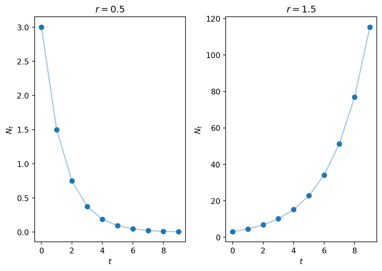
def f(x):
    return r * x

# ------------------------
# Figure setup
# ------------------------
fig, (ax1, ax2) = plt.subplots(1, 2, figsize=(10, 4))

x_full = np.linspace(0, 1.2, 400)

curve_line, = ax1.plot([], [], label="$N_{t+1} = r N_t$")
diag_line, = ax1.plot([], [], '--', label="$N_{t+1} = N_t$")

cobweb_line, = ax1.plot([], [], color='purple', lw=1, label="Cobweb")
point, = ax1.plot([], [], 'ro', markersize=6)

ax1.set_xlim(0, 1.2)
ax1.set_ylim(0, 1.2)
ax1.set_xlabel("$N_t$")
ax1.set_ylabel("$N_{t+1}$")
ax1.set_title("Cobweb diagram")
step_text1 = ax1.text(textPos_x, textPos_y, '', transform=ax1.transAxes,
                     va='top', fontsize=10)
step_text2 = ax1.text(textPos_x-0.15, textPos_y-0.145, '', transform=ax1.transAxes,
                     va='top', fontsize=9.5)                     
ax1.legend(loc='upper left')

time_line, = ax2.plot([], [], 'r-o', markersize=3)
ax2.set_xlim(0, n_steps)
ax2.set_ylim(0, 1.2)
ax2.set_xlabel("t")
ax2.set_ylabel("N")
ax2.set_title("Population vs time")

# ------------------------
# Precompute cobweb + time series
# ------------------------
y_next = f(N0)
xs, ys = [N0], [y_next]
time_vals = [0]
pop_vals = [N0]

x_current = N0
for n in range(1, n_steps):
    xs.append(y_next)
    ys.append(y_next)
    x_current = y_next

    time_vals.append(n)
    pop_vals.append(y_next)

    y_next = f(x_current)
    xs.append(x_current)
    ys.append(y_next)

# ------------------------
# Animation update function
# ------------------------
def update(frame):
    # ---- Phase 1: Draw curves ----
    if frame < n_curve1_frames: # N_t+1 = H(N_t)
        cobweb_line.set_data([],[])
        time_line.set_data([], [])
        k = int(len(x_full) * frame / n_curve1_frames)
        curve_line.set_data(x_full[:k], f(x_full[:k]))
        diag_line.set_data([], [])
        step_text1.set_text("Step 1: Draw $N_{t+1} = H(N_t)$")
        return curve_line, diag_line, cobweb_line, time_line, point, step_text1
    elif frame < n_curve1_frames + wait_frames: # pause
        curve_line.set_data(x_full, f(x_full))
        diag_line.set_data([], [])
        step_text1.set_text("Step 1: Draw $N_{t+1} = H(N_t)$\n"
                           "Step 2: Draw $N_{t+1} = N_t$")
        return curve_line, diag_line, cobweb_line, point, step_text1
    elif frame < n_curve1_frames + n_curve2_frames + wait_frames:  # N_t+1 = N_t
        loc = frame - n_curve1_frames - wait_frames
        k = int(len(x_full) * loc / n_curve2_frames)
        curve_line.set_data(x_full, f(x_full))
        diag_line.set_data(x_full[:k], x_full[:k])
        step_text1.set_text("Step 1: Draw $N_{t+1} = H(N_t)$\n"
                           "Step 2: Draw $N_{t+1} = N_t$")
        return curve_line, diag_line, cobweb_line, point, step_text1
    elif frame < n_curve1_frames + n_curve2_frames + 2*wait_frames: # pause
        curve_line.set_data(x_full, f(x_full))
        diag_line.set_data(x_full, x_full)
        step_text1.set_text("Step 1: Draw $N_{t+1} = H(N_t)$\n"
                       "Step 2: Draw $N_{t+1} = N_t$\n"
                       "Step 3: Mark $(N_0,H(N_0))$")
        return curve_line, diag_line, cobweb_line, point, step_text1
    elif frame < n_curve1_frames + n_curve2_frames + 3*wait_frames: # pause
        curve_line.set_data(x_full, f(x_full))
        diag_line.set_data(x_full, x_full)
        step_text1.set_text("Step 1: Draw $N_{t+1} = H(N_t)$\n"
                       "Step 2: Draw $N_{t+1} = N_t$\n"
                       "Step 3: Mark $(N_0,H(N_0))$\n")
        point.set_data([xs[0]], [ys[0]])
        return curve_line, diag_line, cobweb_line, point, step_text1
    elif frame < n_curve1_frames + n_curve2_frames + 4*wait_frames: # pause
        curve_line.set_data(x_full, f(x_full))
        diag_line.set_data(x_full, x_full)
        step_text1.set_text("Step 1: Draw $N_{t+1} = H(N_t)$\n"
                       "Step 2: Draw $N_{t+1} = N_t$\n"
                       "Step 3: Mark $(N_0,H(N_0))$\n"
                       "Step 4: Horizonatal to red curve\n"
                       "${}_{{{}_{{\scriptscriptstyle \\cdot}}}} \\quad t=1 \\rightarrow (H(N_0),H(N_0))$\n")
        point.set_data([xs[0]], [ys[0]])
        return curve_line, diag_line, cobweb_line, point, step_text1 

    # ---- Phase 2: Cobweb ----
    cobweb_frame = frame - total_curve_frames

    total_segments = n_steps * 2  # 2 per iteration (vertical + horizontal)
    time_progress = n_steps
    # ---- First slow step ----
    if cobweb_frame < first_step_frames:
        progress = cobweb_frame / first_step_frames
        if progress < 0.25:  # horizontal
            p = progress / 0.25
            time_progress = p
            x0, y0, x1, y1 = xs[0], ys[0], xs[1], ys[1]
            x_dot, y_dot = x0 + p*(x1 - x0), y0 + p*(y1 - y0)
            x_draw = [x0, x_dot]
            y_draw = [y0, y_dot]
            step_text1.set_text("Step 1: Draw $N_{t+1} = H(N_t)$\n"
                           "Step 2: Draw $N_{t+1} = N_t$\n"
                           "Step 3: Mark $(N_0,H(N_0))$\n"
                           "Step 4: Horizonatal to red curve\n"
                           "${}_{{{}_{{\scriptscriptstyle \\cdot}}}} \\quad t=1 \\rightarrow (H(N_0),H(N_0))$\n")
        elif progress < 0.75: # pause
            time_progress = 1.0
            x0, y0, x1, y1 = xs[0], ys[0], xs[1], ys[1]
            x_dot, y_dot = x1, y1
            x_draw = [x0, x1]
            y_draw = [y0, y1]
            if progress > 0.3:
              step_text1.set_text("Step 1: Draw $N_{t+1} = H(N_t)$\n"
                           "Step 2: Draw $N_{t+1} = N_t$\n"
                           "Step 3: Mark $(N_0,H(N_0))$\n"
                           "Step 4: Horizonatal to red curve\n"
                           "${}_{{{}_{{\scriptscriptstyle \\cdot}}}} \\quad t=1 \\rightarrow (H(N_0),H(N_0))$\n"
                           "Step 5: Vertical to blue curve\n"
                           "${}_{{{}_{{\scriptscriptstyle \\cdot}}}} \\quad t=1 \\rightarrow (N_1,H(N_1))$\n")
        else: # vertical
            time_progress = 1.0
            p = (progress - 0.75)/0.25
            x0, y0, x1, y1, x2, y2 = xs[0], ys[0], xs[1], ys[1], xs[2], ys[2]
            x_dot, y_dot = x1 + p*(x2 - x1), y1 + p*(y2 - y1)
            x_draw = [x0, x1, x_dot]
            y_draw = [y0, y1, y_dot]
        point.set_data([x_dot], [y_dot])
        cobweb_line.set_data(x_draw, y_draw)
    elif cobweb_frame < first_step_frames + wait_frames:
        time_progress = 1.0
        point.set_data([xs[2]], [ys[2]])
        step_text1.set_text("Step 1: Draw $N_{t+1} = H(N_t)$\n"
                           "Step 2: Draw $N_{t+1} = N_t$\n"
                           "Step 3: Mark $(N_0,H(N_0))$\n"
                           "Step 4: Horizonatal to red curve\n"
                           "${}_{{{}_{{\scriptscriptstyle \\cdot}}}} \\quad t=n \\rightarrow (H(N_{n-1}),H(N_{n-1}))$\n"
                           "Step 5: Vertical to blue curve\n"
                           "${}_{{{}_{{\scriptscriptstyle \\cdot}}}} \\quad t=n \\rightarrow (N_n,H(N_n))$\n")
        step_text2.set_text(r"$\text{Iterate}\left\{ \begin{array}{l} \\ \\ \\ \\ "
                               r" \end{array} \right.$")
    elif cobweb_frame < first_step_frames + wait_frames + remaining_frames:  # remaining frames
        remaining_frame = cobweb_frame - first_step_frames - wait_frames
        remaining_total_frames = remaining_frames
        progress_remaining = remaining_frame / remaining_total_frames

        segments_after_first = xs[2:]  # skip first 2 points
        ys_after_first = ys[2:]

        n_points = int(progress_remaining * (len(segments_after_first)-1))
        n_points = min(n_points, len(segments_after_first)-2)

        x_prev, y_prev = segments_after_first[n_points], ys_after_first[n_points]
        x_next, y_next = segments_after_first[n_points+1], ys_after_first[n_points+1]
        interp = progress_remaining * (len(segments_after_first)-1) - n_points

        x_dot = x_prev + interp*(x_next - x_prev)
        y_dot = y_prev + interp*(y_next - y_prev)

        x_draw = xs[:2] + segments_after_first[:n_points+1] + [x_dot]
        y_draw = ys[:2] + ys_after_first[:n_points+1] + [y_dot]

        point.set_data([x_dot], [y_dot])
        cobweb_line.set_data(x_draw, y_draw)
        if n_points%2 == 0:
          time_progress_int = math.floor(1.0 + (n_steps-2.0)*progress_remaining)
          time_progress_cont = 1.0 + (n_steps-2.0)*progress_remaining - time_progress_int
          time_progress = time_progress_int + 2.0*time_progress_cont
        else:
          time_progress = math.floor(2 + n_points/2.0)

    # ---- Time series ----
    ti = int(math.floor(time_progress))
    tp = time_progress - ti
    t_draw = time_vals[:ti+1]
    p_draw = pop_vals[:ti+1]
    if ti+1 < len(time_vals):
        t0, p0 = time_vals[ti], pop_vals[ti]
        t1, p1 = time_vals[ti+1], pop_vals[ti+1]
        t_draw = list(t_draw) + [t0 + tp*(t1-t0)]
        p_draw = list(p_draw) + [p0 + tp*(p1-p0)]
    time_line.set_data(t_draw, p_draw)

    return curve_line, diag_line, cobweb_line, time_line, point, step_text2

# ------------------------
# Run animation
# ------------------------
ani = animation.FuncAnimation(
    fig,
    update,
    frames=total_frames+final_wait,
    interval=100,
    blit=True
)

if fmt == "html" or fmt is None:
  display(HTML(ani.to_html5_video()))
  plt.close(fig)
else:
  # ---- Render final frame for PDF ----
  update(total_frames + final_wait - 1)
  plt.show()

Figure 2.5: Animation of a cobweb diagram for the Malthusian model with \(N_0 = 0.2\) and \(r = 1.5\).

2.4.5 Bifurcation diagrams

A bifurcation is a qualitative change in solution behaviour as a function of the models parameters (either a change in the number of fixed points or their stability). A bifurcation diagram is a compact means of displaying bifurcations.

The simplest bifurcation digaram is a plot of the fixed point value of the population (which we have often denoted \(N^*\)) against a model parameter of interest. From this diagram one can immediately see how the number of fixed points and their stability changes as a given parameter increases.

2.4.6 Example of a qualitative analysis of the Malhusian model

Let’s work through the various concepts introduced above using the Malthusian model (Equation 2.2).

The fixed points satisfy \[ N^*=rN^*. \tag{2.15}\] As \(r>0\) the only solution is \(N^*=0\).

In this case \[ H'(N_t)=r. \tag{2.16}\] Hence the linear stability of the solution depends on the value of the parameter \(r\) For \(r>1\) the fixed point \(N^*=0\) is monotonically unstable. For \(r<1\) the fixed point \(N^*=0\) is monotonically stable. As expected this result is consistent with the simulation results in Figure 2.1.

For the cobweb diagram:

• Label the axes with \(N_t\) and \(N_{t+1}\).
• From linear stability analysis note there are two qualitatively distinct cases (\(r<1\) and \(r>1\)). We will need a cobweb diagram for each case.
• Case 1: graph the function \(H(N_t)\). In this case it is the straight line \(N_{t+1}=rN_t\) with \(r<1\) (final plot in Figure 2.6).
• Case 2: graph the function \(H(N_t)\). In this case it is the straight line \(N_{t+1}=rN_t\) with \(r>1\) (final plot already shown in Figure 2.5).
• Fill in the cobwebbed trajectories with some arbitrarily chosen initial condition.
• Establish that behaviour of the cobweb is consistent with linear stability analysis.

import numpy as np
import matplotlib.pyplot as plt

# This code computes a cobweb diagram for the Malthusian model

# Define time time vector
T=10
t = np.arange(0, T, 1)

# Define model parameters
N_0=3.0
r=0.5
r_2=1.5

# Define plotting paramneters
N_max=4.0

# define right hand side of malthusian model
def malthusianrhs(x,r):
  f=r*x
  return f

# Compute solution of the difference equation
N,CobwebSol=SolveSingleDiffAndCobweb(t,malthusianrhs,N_0,r)

# Discretise N and plot H
N_plot=np.linspace(0,N_max,100)
H_N_plot=malthusianrhs(N_plot,r)

# Plot results
fig, ax = plt.subplots(1,2)
ax[0].plot(t, N, linestyle='-', alpha=0.4)
ax[0].plot(t, N, linestyle='None', alpha = 1, marker='o', color='C0', ms=3)
ax[0].set_xlabel('$t$')
ax[0].set_ylabel('$N_t$')

ax[1].plot(CobwebSol[:,0], CobwebSol[:,1])
ax[1].plot(CobwebSol[0,0], CobwebSol[0,1],'*')
ax[1].plot([0, N_max], [0, N_max])
ax[1].plot(N_plot, H_N_plot)

ax[1].set_xlabel('$N_t$')
ax[1].set_ylabel('$N_{t+1}$')

plt.tight_layout()

plt.show()

Figure 2.6: A cobweb plot of the Malthusian model solution when \(r\)=0.5. (a) Time series and (b) Cobweb diagrams.

For bifurcation diagram:

• We will plot the value of fixed point against a parameter of interest. In this case \(N^*\) against \(r\).
• Deduce from fixed point and linear stability analysis whether there are any changes in solution behaviour as \(r\) varies (e.g. number of solution or their linear stability).
• In this case the value of the fixed point is independent of \(r\) but the linear stability changes at \(r=1\). This is a bifurcation.
• Use annotation to represent qualitative solution behaviour.

import numpy as np
import matplotlib.pyplot as plt

# Parameter range
r = np.linspace(0, 2.2, 500)

# Equilibrium (N^* = 0)
N_star = np.zeros_like(r)

# Plot
plt.figure(figsize=(8, 5))

# Stable (r < 1)
plt.plot(r[r < 1], N_star[r < 1], 'b', linewidth=3, label='Stable')

# Unstable (r > 1)
plt.plot(r[r > 1], N_star[r > 1], 'r', linewidth=3, label='Unstable')

# Labels
plt.xlabel('r')
plt.ylabel(r'$N^*$')
plt.xlim(-0.05, 2.05) 
plt.title('Bifurcation Diagram of the Malthusian Model')
plt.legend()

plt.show()

Figure 2.7: A bifurcation plot of the Malthusian model as the growth rate \(r\) changes.

2.5 A nonlinear model of population dynamics in discrete time

Consider a model of population growth given by \[ N_{t+1}=\frac{\gamma N_t}{1+N_t^2}, \tag{2.17}\] where \(\gamma\in \Re^+\) is the linear growth rate.

2.5.1 The per capita growth rate

Note that the per capita growth rate is described by the function \[ f(N_{t})=\frac{\gamma}{1+N_t^2}. \tag{2.18}\] Hence at large populations the per capita growth rate tends to zero whilst for small populations it tends to \(\gamma\). Hence so long as \(\gamma>1\) we will have net growth for small populations and net removal for large populations. The net growth rate is given by \[ H(N_{t})=\frac{\gamma N_t}{1+N_t^2}. \tag{2.19}\]

2.5.2 Numerical solution

In Figure 2.8 time series solution of the model are plotted for parameter values \(\gamma=0.5\), \(\gamma=1.5\), \(\gamma=2.5\). Note qualitative changes in model behaviour in the different parameter regimes. Can you identify the fixed points? Are the solutions oscillatory?

# Computes solution of density dependent model
import numpy as np
import matplotlib.pyplot as plt


# Define time
T=10
t = np.arange(0, T, 1)

# Define model parameters
N_0=3.0
gam_1=0.5
gam_2=1.5
gam_3=2.5


# Compute rhs of density dependent model
def densmodelrhs(x,r):
  f=r*x/(1+x**2)
  return f


# Compute solutions for different values of parameter gamma
N_1=SolveSingleDiff(t,densmodelrhs,N_0,gam_1)
N_2=SolveSingleDiff(t,densmodelrhs,N_0,gam_2)
N_3=SolveSingleDiff(t,densmodelrhs,N_0,gam_3)

# PLot results
fig, ax = plt.subplots(1,3)
ax[0].plot(t, N_1, linestyle='-', alpha=0.4)
ax[0].plot(t, N_1, linestyle='None', alpha = 1, marker='o', color='C0', ms=3)
ax[0].set_xlabel('$t$')
ax[0].set_ylabel('$N_{t}$')
ax[1].plot(t, N_2, linestyle='-', alpha=0.4)
ax[1].plot(t, N_2, linestyle='None', alpha = 1, marker='o', color='C0', ms=3)
ax[1].set_xlabel('$t$')
ax[1].set_ylabel('$N_{t}$')
ax[2].plot(t, N_3, linestyle='-', alpha=0.4)
ax[2].plot(t, N_3, linestyle='None', alpha = 1, marker='o', color='C0', ms=3)
ax[2].set_xlabel('$t$')
ax[2].set_ylabel('$N_{t}$')

plt.tight_layout()
plt.show()

Figure 2.8: Time series solution for (a) \(\gamma\)=0.5 and (b) \(\gamma\)=1.5 and (c) \(\gamma\)=10.5.

#| '!! shinylive warning !!': |
#|   shinylive does not work in self-contained HTML documents.
#|   Please set `embed-resources: false` in your metadata.
#| standalone: true
#| components: [viewer]
#| viewerHeight: 500


from shiny import App, Inputs, Outputs, Session, render, ui
from shiny import reactive

import numpy as np
from pathlib import Path
import matplotlib.pyplot as plt
from scipy.integrate import odeint

app_ui = ui.page_fluid(
    ui.layout_sidebar(
        ui.sidebar(
    ui.input_slider(id="r",label="gamma",min=0.0,max=5.0,value=1.2,step=0.001),             
    ui.input_slider(id="u0",label="N_0 (Initial condition)",min=0.0,max=4.0,value=0.5,step=0.01),
    ui.input_slider(id="T",label="Number of iterations",min=0.0,max=60.0,value=20.0,step=1.0),
    ui.input_slider(id="max_sol",label="Max. axis value",min=0.0,max=5.0,value=1.5,step=0.1),

       
        ),

        ui.output_plot("plot"),
    ),
)

def server(input, output, session):
    
    @render.plot
    def plot():
        fig, ax = plt.subplots(2,1)
        #ax.set_ylim([-2, 2])
        # Filter fata
        
        
        r=float(input.r())
        u0=float(input.u0())
        T=int(input.T())
        max_sol=float(input.max_sol())
        
        def rickerrhs(x,par):
          r=par
          K=1.0
          f=r*x/(1+x**2)
          return f
        # Define rhs of logistic map 
     
        # this function computes the solutio to the difference equation. It also stores solution in format for cobweb plotting
        def SolveSingleDiffAndCobweb(t,rhs,N_0,r):
          # Initialise solution vector
          N = np.zeros_like(t,dtype=float)
          N[0]=N_0


          num_time_steps=t.shape[0]


          # Initialise cobweb solution object
          CobwebSol=np.zeros((2*num_time_steps,2))
          CobwebSol[0,0]=N_0
          CobwebSol[0,1]=rhs(N_0,r)
          CobwebSol[1,0]=CobwebSol[0,1]
          CobwebSol[1,1]=CobwebSol[0,1]

          # loop over time and compute solution.
          for i in t:
            if i>0:
              N[i]=rhs(N[i-1],r) 

              sol_temp=N[i-1]
              rhs_temp=rhs(sol_temp,r)
              CobwebSol[2*i,0]=sol_temp
              CobwebSol[2*i,1]=rhs_temp
              CobwebSol[2*i+1,0]=rhs_temp
              CobwebSol[2*i+1,1]=rhs_temp
          return N, CobwebSol

        # Define discretised t domain
        t = np.arange(0, T, 1)
        # define initial conditions
        init_cond=u0
        
        # Compute numerical solution of ODEs
        y,CobwebSol = SolveSingleDiffAndCobweb(t,rickerrhs,init_cond,r)

        # Plot results
        
        ax[0].plot(t, y, linestyle='-', alpha=0.4)
        ax[0].plot(t, y, linestyle='None', alpha = 1, marker='o', color='C0', ms=3)
        ax[0].set_xlabel('$t$')
        ax[0].set_ylabel('$N_t$')
        ax[0].set_title('Time series')

        ax[1].plot(CobwebSol[0,0], CobwebSol[0,1],'*')
        ax[1].plot(CobwebSol[:,0], CobwebSol[:,1],'-')
        ax[1].plot([0,max_sol],[0,max_sol])

        x_plot=np.linspace(0,max_sol,10000)
        y_plot=rickerrhs(x_plot,r)
        ax[1].plot(x_plot,y_plot)
        ax[1].set_title('Cobweb')
        ax[1].set_xlabel('$N_t$')
        ax[1].set_ylabel('$N_{t+1}$')
        ax[1].set_xlim([0,max_sol])

        plt.grid()

        plt.show()
    
app = App(app_ui, server)

Figure 2.9: An app to explore model behaviour.

2.5.3 Fixed points

The fixed points of Equation 2.17 satisfy the algebraic equation \[ N^*=\frac{\gamma N^*}{1+{N^*}^2} \tag{2.20}\] which has solutions \[ N^* = 0 \ \ \ \ \textrm{and} \ \ \ \ N^*=\sqrt{\gamma-1}. \tag{2.21}\]

2.5.3.1 Parameter restrictions for biological validity

If \(\gamma<1\), there is only one biologically relevant fixed point. If \(\gamma >1\) there are two fixed-points, \(N^*=0\) and \(N^*=\sqrt{\gamma-1}\). Hence the value of the model parameter \(\gamma\) qualitatively affects the behaviour and number of solutions.

2.5.4 Linear stability analysis

For the given model we compute \[ H'(N_t)= \frac{\gamma}{1+N_t^2} + \frac{-2 \gamma N_t^2}{(1+N_t^2)^2}. \tag{2.22}\] The stability of the fixed point \(N^*=0\) is determined by \[ H'(0)= \gamma. \tag{2.23}\] Hence if \(\gamma < 1\) the first fixed point is monotonically stable as \(0< H'(0) < 1\). When \(\gamma > 1\) the first fixed point becomes monotonically unstable, also the second fixed point becomes biologically relevant.

The stability of the second fixed point, \(N^*=\sqrt{\gamma-1}\), is determined by

\[\begin{align} H'(\sqrt{\gamma-1})&= \frac{\gamma}{1+\gamma-1} + \frac{-2 \gamma (\gamma-1)}{(1+(\gamma-1))^2}, \\ &= \frac{2}{\gamma}-1. \end{align}\]

Hence the critical point is unstable when, \[ |H'(\sqrt{\gamma-1})| = |\frac{2}{\gamma}-1| >1 \tag{2.24}\] We can show this by considering the two inequalities, \[ \frac{2}{\gamma}-1 > 1 \quad \text{OR} \quad \frac{2}{\gamma}-1 < -1, \] where the first inequality is the condition for montonic unstable and the second oscillatory unstable. The second is never satisfied for \(\gamma > 0\) while the first is satisfied for \(\gamma < 1\). However, a necessary condition for the biological relevance of \(N^*\) is that \(\gamma>1\). Hence \(N^*\), if it is biologically relevant, cannot be unstable.

While \(N^*\) is stable for \(\gamma > 1\), is it montonic or oscillatory? Consider \(H'(N^*)\) and look for sign changes, \[ H'(\sqrt{\gamma-1}) = \frac{2}{\gamma}-1, \] which has a sign change at \(\gamma = 2\) as \(H'(1) = 0\) and the sign changes from positive to negative. Hence \(N^*\) is monotonically stable for \(1 < \gamma < 2\) and is oscillatory stable for \(\gamma > 2\).

Hence, the parameters \(\gamma\) splits the model into three key regimes \(\gamma \in (0,1), \, \gamma \in (1,2), \, \gamma \in (2,\infty)\).

2.5.5 Cobweb diagrams

In Figure 2.10 cobweb diagrams illustrate model behaviour in the three different parameter regimes. Note that the cobweb diagrams can be sketched by hand, given an accurate enough sketch of the right-hand side function \(H(N_t)\). Note also that the cobweb diagrams are consistent with the linear stability analysis but that the linear approximation is only valid close to the equilibrium point.

import numpy as np
import matplotlib.pyplot as plt
from mpl_toolkits.axes_grid1.inset_locator import inset_axes
from matplotlib.lines import Line2D

# Define time vector
T=10
t = np.arange(0, T, 1)

# Define model parameters
N0_list = [1.0, 0.2, 0.2, 0.2]
gamma_list = [0.5, 1.5, 2.5, 3.5]
N_max=4.0

# Solve the model for different values of parameter gamma
solutions = [SolveSingleDiffAndCobweb(t, densmodelrhs, N0_list[i], gamma_list[i]) for i in range(4)]

# Discretise N and plot H for different values of gamma
N_plot = np.linspace(0, N_max, 500) # higher than ussual due to the insets
H_plots = [densmodelrhs(N_plot, gamma) for gamma in gamma_list]

# Plot results
fig, ax = plt.subplots(2, 2, figsize=(10, 8))

# Loop through panels of plots
for i, (axis, (N, Cobweb), H_plot, gamma, N0) in enumerate(zip(
        ax.flatten(), solutions, H_plots, gamma_list, N0_list)):
    # cobweb plot (main plot)
    axis.plot(Cobweb[:,0], Cobweb[:,1])
    axis.plot(Cobweb[0,0], Cobweb[0,1], '*', markersize=8, 
              markerfacecolor='orange', markeredgecolor='orange')  # Initial point star
    axis.plot([0, N_max], [0, N_max])
    axis.plot(N_plot, H_plot)
    axis.set_xlabel('$N_t$')
    axis.set_ylabel('$N_{t+1}$')
    axis.set_title(f'$\gamma = {gamma}$, $N_0 = {N0}$')

    # Compute fixed point
    fixed_point = 0 if gamma <= 1 else np.sqrt(gamma - 1)

    # Compute inset limits
    last_points = Cobweb[-8:, :]
    xmin = min(last_points[:,0].min(), fixed_point)
    xmax = max(last_points[:,0].max(), fixed_point)
    ymin = min(last_points[:,1].min(), fixed_point)
    ymax = max(last_points[:,1].max(), fixed_point)
    xrange = xmax - xmin
    yrange = ymax - ymin
    margin = 0.2 * max(xrange, yrange)
    xmin, xmax = fixed_point - (xrange/2 + margin), fixed_point + (xrange/2 + margin)
    ymin, ymax = fixed_point - (yrange/2 + margin), fixed_point + (yrange/2 + margin)

    # Create inset
    axins = inset_axes(axis, width="40%", height="40%", loc='upper left')
    axins.plot(Cobweb[:,0], Cobweb[:,1])
    axins.plot(Cobweb[0,0], Cobweb[0,1], '*', markersize=8, 
               markerfacecolor='orange', markeredgecolor='orange')  # Star in inset
    axins.plot([0, N_max], [0, N_max])
    axins.plot(N_plot, H_plot)
    axins.plot(fixed_point, fixed_point, 'ro', markersize=6)  # Stable fixed point
    axins.set_xlim(xmin, xmax)
    axins.set_ylim(ymin, ymax)
    axins.set_xticks([])
    axins.set_yticks([])
    axins.set_aspect('equal')

# Add legend at the bottom of the plots
star = Line2D([0], [0], marker='*', color='w', markerfacecolor='orange', markeredgecolor='orange',
              markersize=10, label=r'$(N_0, H(N_0))$')
red_dot = Line2D([0], [0], marker='o', color='w', markerfacecolor='r', markersize=8, label='Stable fixed point')
fig.legend(handles=[star, red_dot], loc='lower center', ncol=2, fontsize=10)

plt.tight_layout(rect=[0, 0.05, 1, 1])  # leave space at bottom for legend
plt.show()

Figure 2.10: Cobweb diagrams for different values of \(\gamma\), along with insets that zoom in on the stable critical point.

2.5.6 Bifurcation diagram

Bifurcations at the critical values \(\gamma=1\) and \(\gamma=2\) are highlighted in the bifurcation diagram presented in Figure 2.11. Note that the bifurcation diagram allows classification of the different model behaviours in a single plot without explicitly calculating the solution to the model.

import numpy as np
import matplotlib.pyplot as plt
from matplotlib.lines import Line2D

# Define gamma regions
gamma_less1 = np.linspace(0, 1, 50) # N^*=0 stable
gamma_greater1 = np.linspace(1, 2, 200) # N^*=0 unstable, non-zero N^* monotonically stable
gamma_greater2 = np.linspace(2, 4, 200) # N^*=0 unstable, non-zero N^* oscillatory stable

# Compute fixed points
N_star_stable0 = np.zeros_like(gamma_less1)
N_star_unstable0 = np.zeros_like(np.concatenate((gamma_greater1
,gamma_greater2)))
N_star_nonzero_mono = np.sqrt(gamma_greater1 - 1)
N_star_nonzero_osc = np.sqrt(gamma_greater2 - 1)

# Plot results
fig, ax = plt.subplots(1)

# Plot N^* = 0 as stable and unstable
ax.plot(gamma_less1, N_star_stable0, 'g') 
ax.plot(np.concatenate((gamma_greater1,gamma_greater2)), N_star_unstable0, 'r')

# Plot N^* = sqrt(gamma-1) as stable
ax.plot(gamma_greater1, N_star_nonzero_mono, 'g')
ax.plot(gamma_greater2, N_star_nonzero_osc, 'b')

# Custom legend
stable_mon_handle = Line2D([0], [0], color='green', lw=2, label='Monotonically stable')
stable_osc_handle = Line2D([0], [0], color='blue', lw=2, label='Oscillatory stable')
unstable_handle = Line2D([0], [0], color='red', lw=2, label=' Unstable')
ax.legend(handles=[stable_mon_handle, stable_osc_handle, unstable_handle], loc='upper left')

plt.xlabel('$\gamma$')
plt.ylabel('$N^*$')
ax.set_title('Bifurcation diagram')
plt.show()

Figure 2.11: A bifiurcation diagram showing how the critical points change.

2.5.7 Symbolic computation

We can use symbolic calculators to aid many of computations performed above. Below is an example using the Python library sympi,

import numpy as np
import sympy as sp

# Define variables and constants
gamma=sp.symbols("gamma",real=True,nonnegative=True)
N = sp.symbols("N",real=True,nonnegative=True)

# Define H
H=gamma*N/(1+N**2)

# Solve the FP equation
fp=sp.solve(H-N,N,dict=True)

print("The FPs are:")
print(fp)

# Compute H prime by differentiating H
H_p=H.diff(N)


print("The derivative of H is:")
print(sp.simplify(H_p))


# Evaluate derivative at different FPs

print("The derivative evaluated at FP 1 is:")
sol1=fp[0][N]
H_p_eval_0=sp.simplify(H_p.subs(N,sol1))

print(H_p_eval_0)

print("The derivative evaluated at FP 2 is:")
sol2=fp[2][N]
H_p_eval_2=H_p.subs(N,sol2)

print(sp.simplify(H_p_eval_2))

The FPs are:
[{N: 0}, {N: -sqrt(gamma - 1)}, {N: sqrt(gamma - 1)}]
The derivative of H is:
gamma*(1 - N**2)/(N**2 + 1)**2
The derivative evaluated at FP 1 is:
gamma
The derivative evaluated at FP 2 is:
(2 - gamma)/gamma

2.6 An application - how much harvesting can a population sustain?

Models of population dynamics can be used to study how interventions will affect population dynamics. Extending from the model developed in the previous example, a valid question might be what is the maximal rate of harvesting a fish stock can sustain without becoming extinct? Introducing a harvesting term at per capita harvesting rate \(h\), the governing model equation becomes \[ N_{t+1}=\frac{\gamma N_t}{1+N_t^2} - h N_t, \tag{2.25}\] which suggests two fundamental questions: (i) does the introduction of harvesting change the dynamics of the system?; and (ii) what rate of harvesting such a population could withstand?

2.6.1 Direct simulation

Based on the previous analysis we consider the system in a parameter regime where without harvesting there is a stable fixed point (\(\gamma>1\)).

import numpy as np
import matplotlib.pyplot as plt

# Define time vector
T=20
t = np.arange(0, T, 1)

# Define model parameters
N_0=0.1
gam=5.0
h_1=0.1
h_2=1.0
h_3=3.0
h_4=5.0

# Define rhs of differnece equation
def densmodelwithharvesting(x,par):
  r=par[0]
  h=par[1]
  f=r*x/(1+x**2)-h*x
  return f

# Compute solution for different values of parameters
N_1=SolveSingleDiff(t,densmodelwithharvesting,N_0,[gam,h_1])
N_2=SolveSingleDiff(t,densmodelwithharvesting,N_0,[gam,h_2])
N_3=SolveSingleDiff(t,densmodelwithharvesting,N_0,[gam,h_3])
N_4=SolveSingleDiff(t,densmodelwithharvesting,N_0,[gam,h_4])

# Plot results
fig, ax = plt.subplots(2,2)
ax[0,0].plot(t, N_1, linestyle='-', alpha=0.4)
ax[0,0].plot(t, N_1, linestyle='None', alpha = 1, marker='o', color='C0', ms=3)
ax[0,0].set_xlabel('$t$')
ax[0,0].set_ylabel('$N_t$')
ax[0,0].set_title(f'$\gamma = ${gam}, $h = ${h_1}')

ax[0,1].plot(t, N_2, linestyle='-', alpha=0.4)
ax[0,1].plot(t, N_2, linestyle='None', alpha = 1, marker='o', color='C0', ms=3)
ax[0,1].set_xlabel('$t$')
ax[0,1].set_ylabel('$N_t$')
ax[0,1].set_title(f'$\gamma = ${gam}, $h = ${h_2}')

ax[1,0].plot(t, N_3, linestyle='-', alpha=0.4)
ax[1,0].plot(t, N_3, linestyle='None', alpha = 1, marker='o', color='C0', ms=3)
ax[1,0].set_xlabel('$t$')
ax[1,0].set_ylabel('$N_t$')
ax[1,0].set_title(f'$\gamma = ${gam}, $h = ${h_3}')

ax[1,1].plot(t, N_4, linestyle='-', alpha=0.4)
ax[1,1].plot(t, N_4, linestyle='None', alpha = 1, marker='o', color='C0', ms=3)
ax[1,1].set_xlabel('$t$')
ax[1,1].set_ylabel('$N_t$')
ax[1,1].set_title(f'$\gamma = ${gam}, $h = ${h_4}')
plt.tight_layout()
plt.show()

Figure 2.12: Time series solution for different values of \(h\).

import numpy as np
import matplotlib.pyplot as plt

# Define time
T=10
t = np.arange(0, T, 1)

# Define parameters
N_0=0.2
h_1=0.1
h_2=1.0
h_3=3.0
h_4=5.0
gamma=5.0

N_max=4.0

# Compute solution at differnet values of h
N1,CobwebSol1=SolveSingleDiffAndCobweb(t,densmodelwithharvesting,N_0,[gamma,h_1])
N2,CobwebSol2=SolveSingleDiffAndCobweb(t,densmodelwithharvesting,N_0,[gamma,h_2])
N3,CobwebSol3=SolveSingleDiffAndCobweb(t,densmodelwithharvesting,N_0,[gamma,h_3])
N4,CobwebSol4=SolveSingleDiffAndCobweb(t,densmodelwithharvesting,N_0,[gamma,h_4])

# Evulate the function H at different values of H
N_plot=np.linspace(0,N_max,100)
H_N_plot1=densmodelwithharvesting(N_plot,[gamma,h_1])
H_N_plot2=densmodelwithharvesting(N_plot,[gamma,h_2])
H_N_plot3=densmodelwithharvesting(N_plot,[gamma,h_3])
H_N_plot4=densmodelwithharvesting(N_plot,[gamma,h_4])

# Plot results
fig, ax = plt.subplots(2,2)

ax[0,0].plot(CobwebSol1[:,0], CobwebSol1[:,1])
ax[0,0].plot(CobwebSol1[0,0], CobwebSol1[0,1],'*')
ax[0,0].plot([0, N_max], [0, N_max])
ax[0,0].plot(N_plot, H_N_plot1)
ax[0,0].set_ylim([-0.001, 4])
ax[0,0].set_xlabel('$N_t$')
ax[0,0].set_ylabel('$N_{t+1}$')
ax[0,0].set_title(f'$\gamma = ${gamma}, $h = ${h_1}')

ax[0,1].plot(CobwebSol2[:,0], CobwebSol2[:,1])
ax[0,1].plot(CobwebSol2[0,0], CobwebSol2[0,1],'*')
ax[0,1].plot([0, N_max], [0, N_max])
ax[0,1].plot(N_plot, H_N_plot2)
ax[0,1].set_ylim([-0.001, 2])
ax[0,1].set_xlabel('$N_t$')
ax[0,1].set_ylabel('$N_{t+1}$')
ax[0,1].set_title(f'$\gamma = ${gamma}, $h = ${h_2}')

ax[1,0].plot(CobwebSol3[:,0], CobwebSol3[:,1])
ax[1,0].plot(CobwebSol3[0,0], CobwebSol3[0,1],'*')
ax[1,0].plot([0, N_max], [0, N_max])
ax[1,0].plot(N_plot, H_N_plot3)
ax[1,0].set_ylim([-0.001, 1])
ax[1,0].set_xlim([-0.001, 2])
ax[1,0].set_xlabel('$N_t$')
ax[1,0].set_ylabel('$N_{t+1}$')
ax[1,0].set_title(f'$\gamma = ${gamma}, $h = ${h_3}')

ax[1,1].plot(CobwebSol4[:,0], CobwebSol4[:,1])
ax[1,1].plot(CobwebSol4[0,0], CobwebSol4[0,1],'*')
ax[1,1].plot([0, N_max], [0, N_max])
ax[1,1].plot(N_plot, H_N_plot4)
ax[1,1].set_ylim([-0.01, 0.01])
ax[1,1].set_xlim([-0.01, 0.01])
ax[1,1].set_xlabel('$N_t$')
ax[1,1].set_ylabel('$N_{t+1}$')
ax[1,1].set_title(f'$\gamma = ${gamma}, $h = ${h_4}')

plt.tight_layout()
plt.show()

Figure 2.13: Cobweb diagrams for different values of \(h\) and \(\gamma = 5\). These are the same values as in Figure 2.12. Note that the scales of the axes are very different in each plot and for \(h = 5\) \(N_1 < 0\) making the cobweb diagram non-physical

#| '!! shinylive warning !!': |
#|   shinylive does not work in self-contained HTML documents.
#|   Please set `embed-resources: false` in your metadata.
#| standalone: true
#| components: [viewer]
#| viewerHeight: 500


from shiny import App, Inputs, Outputs, Session, render, ui
from shiny import reactive

import numpy as np
from pathlib import Path
import matplotlib.pyplot as plt
from scipy.integrate import odeint

app_ui = ui.page_fluid(
    ui.layout_sidebar(
        ui.sidebar(
    ui.input_slider(id="r",label="gamma",min=0.0,max=5.0,value=1.2,step=0.001), 
    ui.input_slider(id="h",label="h",min=0.0,max=5.0,value=1.2,step=0.001),             
    ui.input_slider(id="u0",label="N_0 (Initial condition)",min=0.0,max=4.0,value=0.5,step=0.01),
    ui.input_slider(id="T",label="Number of iterations",min=0.0,max=60.0,value=20.0,step=1.0),
    ui.input_slider(id="max_sol",label="Max. axis value",min=0.0,max=5.0,value=1.5,step=0.1),

       
        ),

        ui.output_plot("plot"),
    ),
)

def server(input, output, session):
    
    @render.plot
    def plot():
        fig, ax = plt.subplots(2,1)
        #ax.set_ylim([-2, 2])
        # Filter fata
        
        
        r=float(input.r())
        h=float(input.h())
        u0=float(input.u0())
        T=int(input.T())
        max_sol=float(input.max_sol())
        
        def rickerrhs(x,r,h):
          f=r*x/(1+x**2)-h*x
          return f
        # Define rhs of logistic map 
     
        # this function computes the solutio to the difference equation. It also stores solution in format for cobweb plotting
        def SolveSingleDiffAndCobweb(t,rhs,N_0,r,h):
          # Initialise solution vector
          N = np.zeros_like(t,dtype=float)
          N[0]=N_0


          num_time_steps=t.shape[0]


          # Initialise cobweb solution object
          CobwebSol=np.zeros((2*num_time_steps,2))
          CobwebSol[0,0]=N_0
          CobwebSol[0,1]=rhs(N_0,r,h)
          CobwebSol[1,0]=CobwebSol[0,1]
          CobwebSol[1,1]=CobwebSol[0,1]

          # loop over time and compute solution.
          for i in t:
            if i>0:
              N[i]=rhs(N[i-1],r,h) 

              sol_temp=N[i-1]
              rhs_temp=rhs(sol_temp,r,h)
              CobwebSol[2*i,0]=sol_temp
              CobwebSol[2*i,1]=rhs_temp
              CobwebSol[2*i+1,0]=rhs_temp
              CobwebSol[2*i+1,1]=rhs_temp
          return N, CobwebSol

        # Define discretised t domain
        t = np.arange(0, T, 1)
        # define initial conditions
        init_cond=u0
        
        # Compute numerical solution of ODEs
        y,CobwebSol = SolveSingleDiffAndCobweb(t,rickerrhs,init_cond,r,h)

        # Plot results
        
        ax[0].plot(t, y, linestyle='-', alpha=0.4)
        ax[0].plot(t, y, linestyle='None', alpha = 1, marker='o', color='C0', ms=3)
        ax[0].set_xlabel('$t$')
        ax[0].set_ylabel('$N_t$')
        ax[0].set_ylim([0,max_sol])
        ax[0].set_title('Time series')


        ax[1].plot(CobwebSol[0,0], CobwebSol[0,1],'*')
        ax[1].plot(CobwebSol[:,0], CobwebSol[:,1],'-')
        ax[1].plot([0,max_sol],[0,max_sol])

        x_plot=np.linspace(0,max_sol,10000)
        y_plot=rickerrhs(x_plot,r,h)
        ax[1].plot(x_plot,y_plot)
        ax[1].set_title('Cobweb')
        ax[1].set_xlabel('$N_t$')
        ax[1].set_ylabel('$N_{t+1}$')
        ax[1].set_xlim([0,max_sol])
        ax[1].set_ylim([0,max_sol])

        plt.grid()

        plt.show()
    
app = App(app_ui, server)

Figure 2.14: An app to explore behaviour in the harvesting model.

In Figure 2.12 time series solutions at increasing harvesting rates (\(h=0.1\), \(h=1\), \(h=3\), \(h=5\)) are presented, and their corresponding cobweb diagrams in Figure 2.13. For low harvesting rates the system behaves almost identically to the no harvesting case but with an expected reduction in the fixed point value. For intermediate harvesting the population undergoes oscillations. However, for further increased harvesting rates there appears again to be a stable fixed point. Eventually we harvest too many fish and the population collapses.

Can analysis of the model help us understand how/why changes in the form of solutions occur?

2.6.2 Fixed points

The fixed points of the system satisfy \[ N^*=\frac{\gamma N^*}{1+{N^*}^2} - h N^*. \tag{2.26}\]

Hence the fixed points are \[ N^*_1=0 \qquad \text{and} \qquad N^*_2=\sqrt{\frac{\gamma}{1+h}-1}. \tag{2.27}\] Note that harvesting lowers the population size of the non-zero fixed point (\(N^*_2\)) when it exists. The condition on the parameters \(\gamma\) and \(h\) in order that there is a non trivial biologically relevant fixed point (\(N^*_2 > 0\)) is given by, \[ \frac{\gamma}{1+h}-1>0 \qquad \Rightarrow \qquad \gamma > 1+h. \tag{2.28}\]

2.6.3 Linear stability

Linear stability is determined by, \[ H'(N_t)=\frac{\gamma}{1+{N_t}^2} - \frac{2\gamma N_t^2 }{(1+{N_t}^2)^2} - h. \tag{2.29}\]

At \(N^*_1=0\) we obtain, \[ H'(0)=\gamma-h. \tag{2.30}\] Hence if \(\gamma>1+h\), \(N^*=0\) is unstable. Note that this is the condition that determines whether the non-zero fixed point \(N^*_2\) exists or not. For the other fixed point \(N_t = N^*_2\) we get, \[ H'\left(\sqrt{\frac{\gamma}{1+h}-1}\right)=\frac{\gamma }{1+\frac{\gamma}{1+h}-1} - \frac{2\gamma \frac{\gamma}{1+h}-1 }{(1+\frac{\gamma}{1+h}-1)^2} - h. \tag{2.31}\] Hence, unsurprisingly, linear stability is now a function of two parameters \(\gamma\) and \(h\). A bit of algebra produces a simpler form as a polynomial in \(h\), \[ H'(N^*_2) = h^2\frac{2}{\gamma} + h\frac{2}{\gamma}(2-\gamma) + \frac{2}{\gamma}-1, \tag{2.32}\] hence when \(h=0\) we retrieve the stability condition from the previous model.

2.6.4 Stability boundaries in the \(h\gamma\) plane

We want to understand the critical points for different parameters choices \((h,\gamma)\). We can break up the \((h,\gamma)\) plane into regions by the contours that determine a change in the linear stability of the critical points. To this end, we want to find the three fundamental contours \(H'(N^*_2)=-1,\, 0,\, 1\) which we do by substituing those values into Equation 2.32, which for our chosen values gives the contours, \[ \begin{aligned} H'(N^*_2) = -1 &\quad \Rightarrow \quad \gamma=\frac{(1+h)^2}{h},\\ H'(N^*_2) = 0 &\quad \Rightarrow \quad \gamma = \frac{2(h+1)^2}{2h+1},\\ H'(N^*_2) = 1 &\quad \Rightarrow \quad \gamma= 1+h, \end{aligned} \tag{2.33}\] All the above analysis can now be summarised by fixing \(h\) where we have the following regions in order of increasing \(\gamma\),

1. \(\boldsymbol{\gamma < h - 1 }\; \Rightarrow \; H'(0) < -1\), \(\, N^*_1\) is oscillatory unstable \(\rightarrow\) population collapse,
2. \(\boldsymbol{h-1 < \gamma < h}\; \Rightarrow \; -1 < H'(0) < 0\), \(\, N^*_1\) is oscillatory stable \(\rightarrow\) population collapse,
3. \(\boldsymbol{h < \gamma < h+1} \; \Rightarrow \; 0 < H'(0) < 1\), \(\, N^*_1\) is monotonically stable \(\rightarrow\) population collapse,
4. \(\boldsymbol{h+1 < \gamma < \frac{2(h+1)^2}{2h+1}} \; \Rightarrow \; 0 < H'(N^*_2) < 1\), $, \(N^*_2\) is monotonically stable \(\rightarrow\) population stable,
5. \(\boldsymbol{\frac{2(h+1)^2}{2h+1}<\gamma <\frac{(1+h)^2}{h}} \; \Rightarrow \; -1 < H'(N^*_2) < 0\), \(\, N^*_2\) is oscillatory stable \(\rightarrow\) population stable,
6. \(\boldsymbol{\gamma >\frac{(1+h)^2}{h}}\; \Rightarrow \; H'(N^*_2) < -1\), \(N^*_2\) is oscillatory unstable \(\rightarrow\) don’t have the tools to know!

In Figure 2.15 we plot the contours of the hypersurface \(H'(N^*)\) at the critical values of \(-1\), \(0\) and 1. Note, that as \(h \rightarrow 0\) we retain the behaviour of the previous model with no harvesting. Also for \(h \gg 3\) the contours all become linear with gradient \(1\). We now understand the long time behaviour of the population unless \(\gamma >\frac{(1+h)^2}{h}\), where \(N^*_2\) is unstable.

Exercise: Consider where in the parameter space the plots in Figure 2.12 and Figure 2.13 are and use this to explain the behaviour of the plots.

In Figure 2.16 we have plotted the time series solution for parameters where \(N^*_2\) is unstable for fixed \(\gamma\). As \(h\) increases the long-time behaviour jumps between 2-values, then jumps between 4-values in a cycle, then it becomes chaotic and finally it returns to a 2-cycle. The next section will attempt to understand this mysterious region.

import numpy as np
import matplotlib.pyplot as plt
import matplotlib.image as mpimg 
from matplotlib.offsetbox import OffsetImage, AnnotationBbox

# Discretize h
h_vec = np.linspace(0.01, 5, 500)

# Compute stability boundaries
gamma_1 = (1 + h_vec)**2 / h_vec      # H_d = -1
gamma_2 = 1 + h_vec                    # H_d = 1
gamma_3 = h_vec                         # N^* = 0 monotonic
gamma_4 = 2 * (1 + h_vec)**2 / (1 + 2*h_vec)  # H_d = 0
gamma_5 = h_vec - 1 # N^* = 0 oscillatory

# Create figure
fig, ax = plt.subplots(figsize=(10,6))
ax.set_ylim(0,12.0)
ax.set_xlim(0,5.0)

# Define colors for regions
colors = {
    'N0_stable': 'lightcoral',
    'nonzero_monot': 'lightgreen',
    'oscillatory': 'lightblue',
    'period_doubling': 'khaki'
}

# Plot shaded regions first
ax.fill_between(h_vec, 0, gamma_5, color='lightcyan', alpha=0.3)
ax.fill_between(h_vec, gamma_5, gamma_3, color=colors['N0_stable'], alpha=0.3)
ax.fill_between(h_vec, gamma_3, gamma_2, color=colors['nonzero_monot'], alpha=0.3)
ax.fill_between(h_vec, gamma_2, gamma_4, color=colors['oscillatory'], alpha=0.3)
ax.fill_between(h_vec, gamma_4, gamma_1, color=colors['period_doubling'], alpha=0.3)
ax.fill_between(h_vec, gamma_1, ax.get_ylim()[1], color='lightgray', alpha=0.3)


# Plot the boundaries with matching colors (darker for contrast)
ax.plot(h_vec, gamma_5, color='purple', lw=2, label="$H'(N_1^*) = -1$")
ax.plot(h_vec, gamma_3, color='darkred', lw=2, label="$H'(N^*_1)=0$")
ax.plot(h_vec, gamma_2, color='darkgreen', lw=2, label="$H'(N^*_2)=1$")
ax.plot(h_vec, gamma_4, color='darkblue', lw=2, label="$H'(N^*_2)=0$")
ax.plot(h_vec, gamma_1, color='goldenrod', lw=2, label="$H'(N^*_2)=-1$")

# Labels and title
ax.set_xlabel('$h$', fontsize=12)
ax.set_ylabel('$\gamma$', fontsize=12)
ax.set_title('Stability Regions', fontsize=14)

# Legend
ax.legend(loc='upper left', bbox_to_anchor=(0.05, 1), fontsize=10)

# Tight layout and grid
plt.tight_layout()
ax.grid(True, linestyle='--', alpha=0.5)

x_0, y_0, x_1, y_1 = 1.0, 1.0, 2.0, 2.0  # data coordinates
x_0_screen, y_0_screen = ax.transData.transform((x_0, y_0))
x_1_screen, y_1_screen = ax.transData.transform((x_1, y_1))
screen_grad = (y_1_screen - y_0_screen)/(x_1_screen - x_0_screen)

# For large h, all slopes ≈ 1
text_angle = np.degrees(np.arctan(screen_grad))
ax.text(3.5, 1.0, '$N^*_1$ oscillatory unstable, population collapse', color='purple', fontsize=10, alpha=1.0)
ax.text(1.5, 0.945, '$N^*_1$ oscillatory stable, population collapse', color='darkred', fontsize=10, alpha=1.0, rotation=text_angle)
ax.text(1.5, 1.945, '$N^*_1$ monotonically stable, population collapse', color='darkgreen', fontsize=10, alpha=1.0, rotation=text_angle)
ax.text(1.5, 2.7, '$N^*_2$ Monotonically stable, population stable', color='darkblue', fontsize=10, alpha=1.0, rotation=text_angle)
ax.text(0.1, 3.4, '$N^*_2$ Oscillatory stable, population stable', color='goldenrod', fontsize=10, alpha=1.0)
ax.text(1.5, 8.5, '$N^*_2$ unstable\n (HERE THERE BE DRAGONS)', color='black', fontsize=10, alpha=1.0, ha='center')

# create dragon image at data point
img = mpimg.imread("./images/dragon.png")
imagebox = OffsetImage(img, zoom=0.15)
ab = AnnotationBbox(imagebox, (3.2, 9.7), frameon=False, xycoords='data')
ax.add_artist(ab)

plt.show()

Figure 2.15: Stability regions from studying the linear stability of the fixed points of the harvesting model. This is not enough to understand population stability/collapse for the grey region, as can be seen in Figure 2.16

import numpy as np
import matplotlib.pyplot as plt

# Define time vector
T=50
t = np.arange(0, T, 1)

# Define model parameters
N_0=0.1
gam=6.0
h_1=0.5
h_2=0.7
h_3=1.2
h_4=3.4

# Define rhs of differnece equation
def densmodelwithharvesting(x,par):
  r=par[0]
  h=par[1]
  f=r*x/(1+x**2)-h*x
  return f

# Compute solution for different values of parameters
N_1=SolveSingleDiff(t,densmodelwithharvesting,N_0,[gam,h_1])
N_2=SolveSingleDiff(t,densmodelwithharvesting,N_0,[gam,h_2])
N_3=SolveSingleDiff(t,densmodelwithharvesting,N_0,[gam,h_3])
N_4=SolveSingleDiff(t,densmodelwithharvesting,N_0,[gam,h_4])

# Plot results
fig, ax = plt.subplots(2,2)
ax[0,0].plot(t, N_1, linestyle='-', alpha=0.4)
ax[0,0].plot(t, N_1, linestyle='None', alpha = 1, marker='o', color='C0', ms=3)
ax[0,0].set_xlabel('$t$')
ax[0,0].set_ylabel('$N_t$')
ax[0,0].set_title(f'$\gamma = ${gam}, $h = ${h_1}')

ax[0,1].plot(t, N_2, linestyle='-', alpha=0.4)
ax[0,1].plot(t, N_2, linestyle='None', alpha = 1, marker='o', color='C0', ms=3)
ax[0,1].set_xlabel('$t$')
ax[0,1].set_ylabel('$N_t$')
ax[0,1].set_title(f'$\gamma = ${gam}, $h = ${h_2}')

ax[1,0].plot(t, N_3, linestyle='-', alpha=0.4)
ax[1,0].plot(t, N_3, linestyle='None', alpha = 1, marker='o', color='C0', ms=3)
ax[1,0].set_xlabel('$t$')
ax[1,0].set_ylabel('$N_t$')
ax[1,0].set_title(f'$\gamma = ${gam}, $h = ${h_3}')

ax[1,1].plot(t, N_4, linestyle='-', alpha=0.4)
ax[1,1].plot(t, N_4, linestyle='None', alpha = 1, marker='o', color='C0', ms=3)
ax[1,1].set_xlabel('$t$')
ax[1,1].set_ylabel('$N_t$')
ax[1,1].set_title(f'$\gamma = ${gam}, $h = ${h_4}')
plt.tight_layout()
plt.show()

Figure 2.16: Time series solution for \(\gamma = 6\) and values of \(h\) inside the grey region of the phase diagram in Figure 2.15 above (where \(N^*_2\) is unstable), demonstrating very different behavour.

Many of the above calculations can be aided using a symbolic calculator:

import numpy as np
import sympy as sp

# Define variables and constants
h=sp.symbols("h",real=True,nonnegative=True)
gamma=sp.symbols("gamma",real=True,nonnegative=True)
N = sp.symbols("N",real=True,nonnegative=True)

# Define H
H=gamma*N/(1+N**2)-h*N

# Solve the FP equation
fp=sp.solve(H-N,N,dict=True)

print("The FPs are:")
print(fp[0])
print(fp[1])
print(fp[2])

# Compute H prime
H_p=H.diff(N)

print("The derivative of H is:")
print(sp.simplify(H_p))

# Evaluate derivative

print("The derivative evaluated at FP 0 is:")
sol1=fp[0][N]
H_p_eval_0=sp.simplify(H_p.subs(N,sol1))

print(H_p_eval_0)

print("The derivative evaluated at FP 2 is:")
sol2=fp[2][N]
H_p_eval_2=H_p.subs(N,sol2)

print(sp.simplify(H_p_eval_2))

The FPs are:
{N: 0}
{N: -sqrt(gamma - h - 1)/sqrt(h + 1)}
{N: sqrt(gamma - h - 1)/sqrt(h + 1)}
The derivative of H is:
-N**2*gamma/(N**2 + 1)**2 + gamma/(N**2 + 1)**2 - h
The derivative evaluated at FP 0 is:
gamma - h
The derivative evaluated at FP 2 is:
(gamma + 2*(h + 1)*(-gamma + h + 1))/gamma

2.7 Oscillations, \(n\)-cycles and chaos

Linear stability analysis describes the evolution of small perturbations close to a fixed point. But far from a fixed point the nonlinear terms that were dropped in a Taylor expansion are no longer negligible. In particular, in the case where \(H'(N^*)<-1\), it can be the case that regions of parameter space in which a fixed point is oscillatory unstable can give rise to periodic and chaotic solutions.

Consider a general difference equation of the form, \[ N_{t+1}=H(N_t) \tag{2.34}\] A solution to Equation 2.34 is defined to be periodic with period \(T\) if and only if, \[ \begin{aligned} N_{t+T}&=N_t& \forall t,\\ N_{t+\tau}&\neq N_t& \forall t, \end{aligned} \tag{2.35}\] where \(\tau < T\).

Period 2 solutions or 2-cycles can be identified by looking for solutions that repeat after two iterations, hence a population \(\bar{N}\) defines a 2-cycle if and only if, \[ \bar{N} = H(H(\bar{N})) = H^2(\bar{N}), \quad \text{where} \, \bar{N} \neq H(\bar{N}), \tag{2.36}\] Hence, we can define a general \(n\)-cycle as \(\bar{N}\) such that, \[ \bar{N} = H^n(\bar{N}), \quad \text{where} \, \bar{N} \neq H^k(\bar{N}) \; \forall \, k\in \mathbb{N}, \, k < n. \tag{2.37}\] Hence, \(n\)-cycles are fixed points of the problem, \[ N_{t+n}=H^n(N_t). \tag{2.38}\] Note that finding a fixed point of Equation 2.38 is not sufficient to show it is an \(n\)-cycle as it must also not be a fixed point of \(N_{t+k} = H^k(N_t)\) where \(0 < k < n\). For example, fixed points of \(H(N_t)\) are all fixed points of \(H^n(N_t)\; \forall \, n\in\mathbb{N}\).

We have already developed the tools to find such fixed points and study their stability. Note that as the period of the solutions increases the right hand side of the function becomes increasingly complicated to tackle algebraically.

2.7.1 The harvesting model revisted

In many systems, such as the harvesting model and the logistic equation, increasing the growth rate parameter leads initially to the fixed point becoming unstable and the emergence of period two solutions, then period 4 solutions and so on until eventually there is a transition to chaotic solutions.

Consider period 2 solutions \(\bar{N}\) of Equation 2.25, namely solutions of, \[ \bar{N} = H^2(\bar{N}) = \frac{\gamma \frac{\gamma\bar{N}}{1+\bar{N}^2}-h\bar{N}}{1 + \left( \frac{\gamma\bar{N}}{1+\bar{N}^2}-h\bar{N} \right)^2} - h \frac{\gamma\bar{N}}{1+\bar{N}^2}-h\bar{N}. \tag{2.39}\] This is certainly solvable by hand but is easier using SymPy which we do below. We simplified Equation 2.39 so it became a degree 9 polynomial in \(\bar{N}\). We already know some of the roots however, as all 1-cycles (fixed points of \(H\)) will be fixed points of \(H^2\). So we can divide by these three roots simplifying to a sextic but with even powers only. Hence we end up with a cubic in \(\bar{n} = \bar{N}^2\), which we can solve. We then select only positive cycles \((\bar{N}_1, \bar{N_2})\) such that, \[ \bar{N}_1 = H(\bar{N}_2), \quad \text{and} \; \bar{N}_2 = H(\bar{N}_1). \tag{2.40}\] Note that the pair \((-\bar{N}_1, -\bar{N_2})\) will always exist due to the symmetry of the polynomial.

Finally we now consider the stability of each fixed point, which is given by \((H^2)'(\bar{N}_1)\) which is simply given by the chain rule to be, \[ (H^2)'(\bar{N}_1) = H'(H(\bar{N}_1))H'(\bar{N}_1) = H'(\bar{N}_2)H'(\bar{N}_1), \tag{2.41}\] which is equivalent for \((H^2)'(\bar{N}_2)\). In Figure 2.17 we then plot three regions in the \((h,\gamma)\) plane,

• discriminant of the quadratic \(\Delta(\bar{n}) < 0\), hence no real solutions and no physical 2-cycle (grey),
• \(0 < H'(\bar{N}_1)H'(\bar{N}_2) < 1\), hence the 2-cycle is monotonically stable (blue),
• \(-1 < H'(\bar{N}_1)H'(\bar{N}_2) < 0\), hence the 2-cycle is oscillatory stable (green),
• \(H'(\bar{N}_1)H'(\bar{N}_2) < -1\), hence the 2-cycle is oscillatory unstable (red).

import numpy as np
import sympy as sp
import matplotlib.pyplot as plt

# Define variables and constants
h=sp.symbols("h",real=True,nonnegative=True)
gamma=sp.symbols("gamma",real=True,nonnegative=True)
N = sp.symbols("N",real=True,nonnegative=True)

# Define H
H=gamma*N/(1+N**2)-h*N

# Define H squared - N
Hsq=gamma*H/(1+H**2)-h*H
Hsq_minN=gamma*H/(1+H**2)-h*H - N
# multiply through by the denominators and simplify
Hsq_minN_simp=sp.simplify(Hsq_minN*(1+H**2)*(1+N**2)**3)

# Solve the FP equation
fp=sp.solve(H-N,N,dict=True)

print("The FPs are:")
print(fp[0])
print(fp[1])
print(fp[2])

# Compute H prime
H_p=H.diff(N)

print("The derivative of H is:")
print(sp.simplify(H_p))

# Evaluate derivative

print("The derivative evaluated at FP 0 is:")
sol1=fp[0][N]
H_p_eval_0=sp.simplify(H_p.subs(N,sol1))
print(H_p_eval_0)

print("The derivative evaluated at FP 2 is:")
sol2=fp[2][N]
H_p_eval_2=H_p.subs(N,sol2)
print(sp.simplify(H_p_eval_2))

# factor out N = 0 fixed point
Q_N = sp.simplify(Hsq_minN_simp / N)

# substitute in n = N^2 as this is a polynomial in N^2
n = sp.symbols("n", real=True, nonnegative=True)
Q_n = sp.expand(Q_N.subs(N, sp.sqrt(n)))
Q_n_simp = sp.simplify(Q_n)

n_fp = fp[2][N]**2
Q_n_simp = sp.simplify(sp.expand(Q_n_simp)/(n-n_fp))

print("The 2-cycle polynomial is:")
print(sp.factor(Q_n_simp))

# Solve the cubic for n
solutions_n = sp.solve(Q_n_simp, n)

# Remove any negative solutions (since n = N^2 >= 0)
solutions_n = [sol for sol in solutions_n]

# Recover N values
print("with solutions:")
N_vals = []
for n_val in solutions_n:
    print(n_val)
    N_vals.append(sp.simplify(sp.sqrt(n_val)))
    N_vals.append(sp.simplify(-sp.sqrt(n_val)))
    
physical_solutions = []
    
print("solutions with non-physical 2-cycles:")
for n_val in solutions_n:
    N1 = sp.sqrt(n_val)
    N2 = -sp.sqrt(n_val)
    # Check if the pair gives a valid 2-cycle
    H_N1 = H.subs(N, N1)
    H_N2 = H.subs(N, N2)
    if sp.simplify(H_N1 - N2) != 0:
        # Only keep the solution if it is a physical 2-cycle
        physical_solutions.append(n_val)
    else:
        print(n_val)
        
# Reconstruct a polynomial with these roots
poly_phys = 1
for root in physical_solutions:
    poly_phys *= (n - root)

# Expand to get a proper polynomial
poly_phys = sp.expand(poly_phys)
poly_phys_poly = sp.Poly(poly_phys, n)
disc_phys = sp.simplify(sp.discriminant(poly_phys_poly, n))

print("Discriminant of the physical 2-cycle polynomial:")
print(disc_phys)

N1 = np.abs(sp.sqrt(physical_solutions[0]))
N2 = np.abs(H.subs(N, N1))
stability_expr = sp.simplify(H_p.subs(N, N1) * H_p.subs(N, N2))

multiplier_func = sp.lambdify((h, gamma), stability_expr, 'numpy')
N1_func = sp.lambdify((h, gamma), N1, 'numpy')
N2_func = sp.lambdify((h, gamma), N2, 'numpy')

# set up plot
h_vals = np.linspace(0.01, 5, 3000) # avoid h=0 to prevent division by zero
gamma_vals = np.linspace(0.01, 12, 3000)
H_grid, G_grid = np.meshgrid(h_vals, gamma_vals)

M = multiplier_func(H_grid, G_grid)
N1_grid = np.real(N1_func(H_grid, G_grid))
N2_grid = np.real(N2_func(H_grid, G_grid))

# Mask for physical 2-cycles
mask = (N1_grid > 0) & (N2_grid > 0) & np.isfinite(M)
M_masked = np.where(mask, M, np.nan)

# Define the regions
stable_monotonic   = np.where((M_masked > 0) & (M_masked < 1), 1, np.nan)
stable_oscillatory = np.where((M_masked < 0) & (M_masked > -1), 1, np.nan)
unstable_monotonic = np.where(M_masked >= 1, 1, np.nan)
unstable_oscillatory = np.where(M_masked <= -1, 1, np.nan)

disc_func = sp.lambdify((h, gamma), disc_phys, 'numpy')
D = disc_func(H_grid, G_grid)
no_cycle_mask = D < 0 # True where 2-cycle does NOT exist

plt.figure(figsize=(10,6))

# Contours for multiplier -1, 0, 1
levels = [-1, 0.0, 0.983]
contour = plt.contour(H_grid, G_grid, M, levels=levels, colors=['darkred', 'darkgreen', 'darkblue'], linewidths=2)

# Fill stable regions
plt.contourf(H_grid, G_grid, stable_monotonic, levels=[0,1], colors=['lightblue'], alpha=0.3)
plt.contourf(H_grid, G_grid, stable_oscillatory, levels=[0,1], colors=['lightgreen'], alpha=0.3)

# Fill unstable regions
plt.contourf(H_grid, G_grid, unstable_oscillatory, levels=[0,1], colors=['lightcoral'], alpha=0.3)
plt.contourf(H_grid, G_grid, no_cycle_mask, levels=[0,1], colors=['lightgray'], alpha=0.3, extend='both')

plt.xlabel('h')
plt.ylabel('$\gamma$')
plt.title('Stability regions of physical 2-cycles')
plt.grid(True, linestyle='--', alpha=0.5)

# Create custom legend for contours and regions
from matplotlib.lines import Line2D

# Contour lines for the legend only
red_line   = Line2D([0], [0], color='darkred',   lw=2, label=r"$H'(\bar{N}_1) H'(\bar{N}_2) = -1$")
green_line = Line2D([0], [0], color='darkgreen', lw=2, label=r"$H'(\bar{N}_1) H'(\bar{N}_2) = 0$")
blue_line  = Line2D([0], [0], color='darkblue',  lw=2, label=r"$H'(\bar{N}_1) H'(\bar{N}_2) = 1$")

# Create custom legend for contours and regions
import matplotlib.patches as mpatches
light_blue = mpatches.Patch(color='lightblue', alpha=0.3, label='Stable 2-cycle (monotonic)')
light_red = mpatches.Patch(color='lightcoral', alpha=0.3, label='Unstable 2-cycle (oscillatory)')
light_green = mpatches.Patch(color='lightgreen', alpha=0.3, label='Stable 2-cycle (oscillatory)')
light_grey = mpatches.Patch(color='lightgray', alpha=0.3, label='No real solutions')

plt.legend(handles=[red_line, green_line, blue_line, light_red, light_green, light_blue, light_grey], loc='upper right')

plt.show()

The FPs are:
{N: 0}
{N: -sqrt(gamma - h - 1)/sqrt(h + 1)}
{N: sqrt(gamma - h - 1)/sqrt(h + 1)}
The derivative of H is:
-N**2*gamma/(N**2 + 1)**2 + gamma/(N**2 + 1)**2 - h
The derivative evaluated at FP 0 is:
gamma - h
The derivative evaluated at FP 2 is:
(gamma + 2*(h + 1)*(-gamma + h + 1))/gamma
The 2-cycle polynomial is:
(h + 1)*(-gamma + h*n + h - n - 1)*(-gamma*h*n + h**2*n**2 + h**2*n + n + 1)
with solutions:
(gamma*h - h**2 - sqrt(gamma**2*h**2 - 2*gamma*h**3 - 2*gamma*h + h**4 - 2*h**2 + 1) - 1)/(2*h**2)
(gamma*h - h**2 + sqrt(gamma**2*h**2 - 2*gamma*h**3 - 2*gamma*h + h**4 - 2*h**2 + 1) - 1)/(2*h**2)
(gamma - h + 1)/(h - 1)
solutions with non-physical 2-cycles:
(gamma - h + 1)/(h - 1)
Discriminant of the physical 2-cycle polynomial:
gamma**2/h**2 - 2*gamma/h - 2*gamma/h**3 + 1 - 2/h**2 + h**(-4)

Figure 2.17: The regions of stability of fixed points of period 2 or 2-cycles.

(see, for example, Figure 2.18).

import numpy as np
import matplotlib.pyplot as plt

# Define time

T=40
t = np.arange(0, T, 1)

# Define model parameters
N_0=0.1
r_1=9.68
r_2=12.221
r_3=30.25
h=0.1

# Plotting parameters
N_max=20.0


# Solve model and compuote cobweb data

N1,CobwebSol1=SolveSingleDiffAndCobweb(t,densmodelwithharvesting,N_0,[r_1,h])
N2,CobwebSol2=SolveSingleDiffAndCobweb(t,densmodelwithharvesting,N_0,[r_2,h])
N3,CobwebSol3=SolveSingleDiffAndCobweb(t,densmodelwithharvesting,N_0,[r_3,h])


# Discretise N and generate H for different values of r
N_plot=np.linspace(0,N_max,100)
H_N_plot1=densmodelwithharvesting(N_plot,[r_1,h])
H_N_plot2=densmodelwithharvesting(N_plot,[r_2,h])
H_N_plot3=densmodelwithharvesting(N_plot,[r_3,h])


# Make figure
fig, ax = plt.subplots(3,2)

ax[0,0].plot(t, N1, linestyle='-', alpha=0.4)
ax[0,0].plot(t, N1, linestyle='None', alpha = 1, marker='o', color='C0', ms=3)
ax[0,0].set_xlabel('$t$')
ax[0,0].set_ylabel('$N_{t}$')

ax[0,1].plot(CobwebSol1[:,0], CobwebSol1[:,1])
ax[0,1].plot(CobwebSol1[0,0], CobwebSol1[0,1],'*')
ax[0,1].plot([0, N_max], [0, N_max])
ax[0,1].plot(N_plot, H_N_plot1)
ax[0,1].set_xlabel('$N_t$')
ax[0,1].set_ylabel('$N_{t+1}$')

ax[1,0].plot(t, N2, linestyle='-', alpha=0.4)
ax[1,0].plot(t, N2, linestyle='None', alpha = 1, marker='o', color='C0', ms=3)
ax[1,0].set_xlabel('$t$')
ax[1,0].set_ylabel('$N_{t}$')

ax[1,1].plot(CobwebSol2[:,0], CobwebSol2[:,1])
ax[1,1].plot(CobwebSol2[0,0], CobwebSol2[0,1],'*')
ax[1,1].plot([0, N_max], [0, N_max])
ax[1,1].plot(N_plot, H_N_plot2)
ax[1,1].set_xlabel('$N_t$')
ax[1,1].set_ylabel('$N_{t+1}$')

ax[2,0].plot(t, N3, linestyle='-', alpha=0.4)
ax[2,0].plot(t, N3, linestyle='None', alpha = 1, marker='o', color='C0', ms=3)
ax[2,0].set_xlabel('$t$')
ax[2,0].set_ylabel('$N_{t}$')

ax[2,1].plot(CobwebSol3[:,0], CobwebSol3[:,1])
ax[2,1].plot(CobwebSol3[0,0], CobwebSol3[0,1],'*')
ax[2,1].plot([0, N_max], [0, N_max])
ax[2,1].plot(N_plot, H_N_plot3)
ax[2,1].set_xlabel('$N_t$')
ax[2,1].set_ylabel('$N_{t+1}$')
plt.tight_layout()

plt.show()

Figure 2.18: Transition form period 2 to period 4 solutions in the harvesting model

We could repeat the above process for 4-cycles and then 8-cycles though it will get progressively harder. To get a feel for what happens as the harvesting rate increases in this region we could instead do some numerics to simulate a bifurcation diagram. Here we plot all possible final populations for each \(h\), namely all \(N_t\) for \(300 < t < 800\). The results of this are shown in Figure 2.19, where we can see for \(\gamma = 6\) as \(h\) increases from 0 and decreases from 4 the period of the solution doubles with decresing interval and then becomes chaotic. There are also large white regions amonst the chaos, where ordered dynamics returns before becoming chaotic again. These kind of features appear in many non-linear population models.

import numpy as np
import matplotlib.pyplot as plt

# Parameters
gamma_vals = [4.0, 5.0, 6.0, 7.0]  # different fixed gamma
h_vals = np.linspace(0, 5, 2000)    # vary h
N0 = 0.1                             # initial condition
transient = 300                      # iterations to discard
iterations = 800                     # total iterations

# function H(N)
def H(N, h, gamma):
    return gamma * N / (1 + N**2) - h * N

# create figure
fig, axes = plt.subplots(2, 2, figsize=(12, 10))
axes = axes.flatten()

# loop through fixed gamma values
for idx, gamma_val in enumerate(gamma_vals):
    ax = axes[idx]
    # loop through h
    for h in h_vals:
        N = N0
        trajectory = []
        # iterate H(N)
        for i in range(iterations):
            N = H(N, h, gamma_val)
            if i >= transient:
                trajectory.append(N)
        # plot bifurcation points
        ax.plot([h]*len(trajectory), trajectory, ',k', markersize=4, alpha=0.7)
    
    ax.set_title(f'$\gamma = ${gamma_val}')
    ax.set_xlim(0, 5)
    ax.set_ylim(0, 3)
    ax.set_xlabel('$h$')
    ax.set_ylabel('$N_{\infty}$')
    ax.grid(True, linestyle='--', alpha=0.5)

plt.tight_layout()
plt.show()

Figure 2.19: Bifurcation diagram showing how possible long time populations \(N_\infty\) change for \(t > 300\) with \(h\) for various values of fixed \(\gamma\) and varying \(h\).

2.8 A note on the modelling of real-world fish stocks

You can find reports on fish stocks (measurements and modelling work) from the International Council for the Exploration of the Sea at the link. Here’s a link to the data for Atlantic salmon. Note that although the models we have worked on are not detailed enough to accurately model real fish population dynamics, many of the principles we have covered arise in the cutting edge models.