4  Single species population dynamics

In this chapter we define time, \(t\), to be a continuous variable and the population density, \(N(t)\), to represent the size of a given population.

4.1 The Malthusian (linear) model

As time is now a continuous variable, we consider an interval of time \(\delta t\). Consider a population of size \(N(t)\). If the per capita production rate is \(b\), then in time \(\delta t\) the increase in population size will be \[ b N(t) \delta t. \tag{4.1}\] Similarly, if the per capita death rate is \(d\), the decrease in population size in time \(\delta t\) will be \[ d N(t) \delta t. \tag{4.2}\] Hence \[ N(t+\delta t)= N(t) + (bN(t)-dN(t))\delta t. \tag{4.3}\] Rearranging and taking the limit as \(\delta t \rightarrow 0\) yields \[ \frac{dN}{dt}=(b-d)N=rN(t). \tag{4.4}\]

The solution can be found using seperation of variables, \[ N(t)=N_0\exp(rt), \tag{4.5}\] where \(N_0\) is the initial population at time \(t=0\). We can describe qualitatively different solutions behaviours,

• \(r>0\), the solution increases exponentially,
• \(r<0\), the solution decreases exponentially,
• \(r=0\), the solution is constant.

Malthusian growth in the continuous time model leads to either a constant population, exponentially increasing or exponentially decreasing growth. As was the case for the discrete time model, such a model could account for biological system only in particularly limited circumstances.

The Malthusian model (constant per capita growth rate) can exhibit a limited range of behaviour. To account for limitation of population growth at large population densities due to, for example, limited resources, we consider nonlinear per capita growth rates.

4.2 Tools for analysing the dynamics of a single population in continuous time

Let \(N=N(t)\). We consider the general form for a single species model defined in continuous time, \[ \frac{dN}{dt}=f(N)N=H(N), \tag{4.6}\] where \(f\) is the per capita growth rate and \(H\) is the net growth rate.

4.2.1 Numerical solution

Although an equation of the form Equation 4.6 may not be explicitly integrable, so long as the right-hand side is sufficiently well behaved, we can numerically integrate the problem (e.g. using packages such as Python’s odeint). Such a technique provides a numerical approximation to the exact solution, given specific values of model parameters and initial conditions (i.e. we can graph solutions).

4.2.2 Steady-state

We denote steady-state solutions or equilibria of Equation 4.6 using \(N=N^*\). At a steady-state, \[ \frac{dN}{dt}=0, \tag{4.7}\] and hence steady-states can be obtained by solving the algebraic equation, \[ H(N^*)=0. \tag{4.8}\] Note, some texts may call these fixed points or critical points. The first is often used in dynamical systems, while the second is older and rarely used as it can be ambiguous.

4.2.3 Linear stability analysis

To perform a linear stability analysis near an equillibrium we make the change of variables, \[ N(t)=N^*+\hat{N}(t), \tag{4.9}\] where the new dependent variable, \(\hat{N}(t)\), is a perturbation about the steady state \(N^*\). The time derivative on the left-hand side of Equation 4.6 transforms to, \[ \frac{dN}{dt}= \frac{d }{dt} (N^*) + \frac{d }{dt}(\hat{N}(t))=\frac{d\hat{N}(t) }{dt}. \tag{4.10}\] Hence Equation 4.6 transforms to \[ \frac{d\hat{N}(t) }{dt} = H(N^*+\hat{N}(t)). \tag{4.11}\]

Employing a Taylor expansion on the right-hand side of Equation 4.6 we get, \[ \frac{d\hat{N}(t) }{dt} = H(N^*)+ H'(N^*)\hat{N}(t) + \frac{1}{2}H''(N^*)\hat{N}^2(t) + \mathcal{O}(\hat{N}^3), \tag{4.12}\] where we use \(H(N^*)=0\) and assume the perturbation \(\hat{N}\) is small to neglect all terms quadratic and higher, which yields the linear ODE, \[ \frac{d\hat{N}(t) }{dt} = H'(N^*)\hat{N}(t) \tag{4.13}\] with solution (by separation of variables), \[ \hat{N}(t)= \eta e^{H'(N^*) t} \tag{4.14}\] where \(\eta\) is some initial perturbation about the steady-state. We now have 3 phases in this linear regime,

• \(H'(N^*)>0,\) the pertubration grows exponentially fast and the steady-state is unstable.
• \(H'(N^*)<0,\) the perturbation decays exponentially fast and the steady-state is stable.
• \(H'(N^*)=0,\) the marginal case where linearisation is inconclusive and higher-order terms determine stability.

Note that, for the discrete time case, our solutions could decay or grow montonically or oscillatory. This is no longer the case for the continous model (as it would require \(H'(N^*)\) to change in time). So we only have monotonic decay or growth.

4.2.4 Graphical solution

We can graphically identify steady-states and their stability by plotting \(dN/dt\) against \(N(t)\). Steady-states arise at the roots of \(H(N)\). The sign of the derivative at a root determines its linear stability.

4.2.5 Bifurcation diagrams

Bifurcations arise when the number of solutions or their stability changes at a given value of a model parameter. By plotting the steady state solutions against a model parameter and using annotation to represent stability of solutions we can obtain a bifurcation diagram.

As an exercise perform a qualitative analysis of the Malthusian model.

4.3 The logistic growth model

4.3.1 Model development

Let \(N=N(t)\). The logistic model, due to Verhulst, takes the form \[ \frac{dN}{dt}=rN(t)\left (1-\frac{N(t)}{K}\right), \tag{4.15}\]

where \(r\) is the linear growth rate and \(K\) is carrying capacity. We consider both \(r,K\in \Re^+\).

Questions to ask of such a model are: what type of biologically realistic solutions does it possess? Are there steady-states? If so, are they stable or unstable? Are there bifurcations in solutions?

4.3.1.1 Numerical solutions

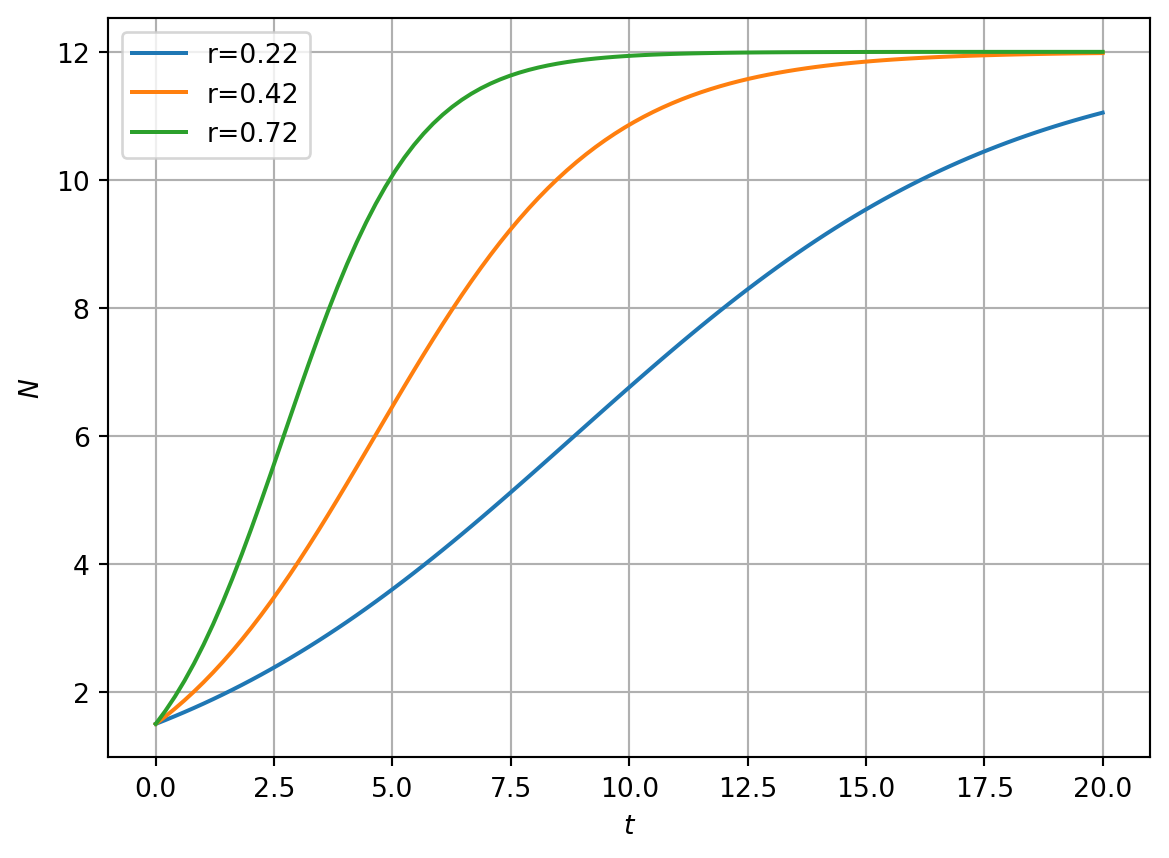
In Figure 4.1 we present numerical solutions of equation using different initial conditions. Note the limiting behaviour of solutions as \(t\rightarrow \infty\). In Figure 4.1 it is clear that even though some solutions are initialised at \(N_0=0.1\), much closer to \(N^*=0\) than \(N^*=K\), they tend to the limit \(N=K\). Why do solutions not tend to \(N^*=0\)?

import numpy as np
import matplotlib.pyplot as plt
import scipy
from scipy.integrate import odeint
# This codes computes a numerical solution of the logistic growth model


# Define model parameters
K=12
r_1=0.22
r_2=0.42
r_3=0.72

# Plotting parameter
N_max=1.1

# Initial condition
n_0=1.5
# Max time
T=20
t=np.linspace(0,T,100)

def rhslogistic_model(x,t,r,K):

  rhs=r*x*(1-x/K)
  return rhs

# Numerically solve the ODE for different parameter values
sol1=odeint(rhslogistic_model,n_0,t,args=(r_1,K))
sol2=odeint(rhslogistic_model,n_0,t,args=(r_2,K))
sol3=odeint(rhslogistic_model,n_0,t,args=(r_3,K))


# Plot solutions
fig, ax = plt.subplots(1)

ax.plot(t, sol1,t, sol2,t, sol3)
plt.xlabel('$t$')
plt.ylabel('$N$')
plt.grid(True)
plt.legend(['r='+str(r_1),'r='+str(r_2),'r='+str(r_3)])
plt.show()

Figure 4.1: Numerical solution of the logistic growth model

4.3.1.2 Dimensional analysis and nondimensionalisation

\(N\) represents the population density and has units of one over area (say \(1/m^2\)) and \(t\) has units of time (say, seconds, \(s\)). Hence the left-hand side of Equation 4.15 has units of \(1/(m^2 s)\). The first term on the right-hand side of Equation 4.15 is \(rN\). \(N\) has units \(1/m^2\) hence the parameter \(r\) must have units of \(1/s\) for dimensional consistency. This is consistent as \(r\) represents the linear growth rate.

The second term has the form \(rN^2/K\). Given the chosen units for \(r\) and \(N\), the parameter \(K\) must have dimensions \(1/m^2\). Again, this is consistent as \(K\) is a carrying capacity (i.e. it has units of population density).

We define the nondimensionalised variables \[ n=\frac{N}{\tilde{N}} \ \ \ \ \ \ \tau=\frac{t}{\tilde{T}} \tag{4.16}\] where \(\tilde{N}\) and \(\tilde{T}\) are constants that have units of population density and time, respectively. Hence Equation 4.15 transforms, upon change of variables, to \[ \begin{aligned} \frac{\tilde{N}}{\tilde{T} }\frac{dn}{d\tau}=r\tilde{N}n(1-\frac{n\tilde{N}}{K}). \end{aligned} \tag{4.17}\]

In the case of the logistic equation there is only one time scale and density scale in the problem, hence we choose \[ \tilde{T}=\frac{1}{r} \ \ \ and \ \ \ \tilde{N}=K \tag{4.18}\] and the dimensionless model is \[ \begin{aligned} \frac{dn}{d\tau}= n(1-n) \end{aligned} \tag{4.19}\] Note that we can retrieve the original equation by rescaling and calculating \(N=\tilde{N}n\) and \(t=\tilde{T}\tau\).

4.3.2 Steady states and linear stability

Steady states satisfy \[ n^*(1-n^*)=0. \tag{4.20}\] Hence \[ n^*=0, \ \ \ \ n^*=1. \tag{4.21}\]

To determine linear stability we compute \[ H'(n)= (1-2n). \tag{4.22}\] When \(n=n^*=0\) we obtain \[ H'(n)= 1. \tag{4.23}\] Hence the origin is an unstable steady-state.

At the steady-state \(n^*=1\) \[ H'(n^*)= -1 \tag{4.24}\] hence \(n^*=1\) is linearly stable.

Note that the linear stability analysis can explain the observations regarding the numeric solutions presented in Figure 4.1.

4.3.3 Graphical analysis

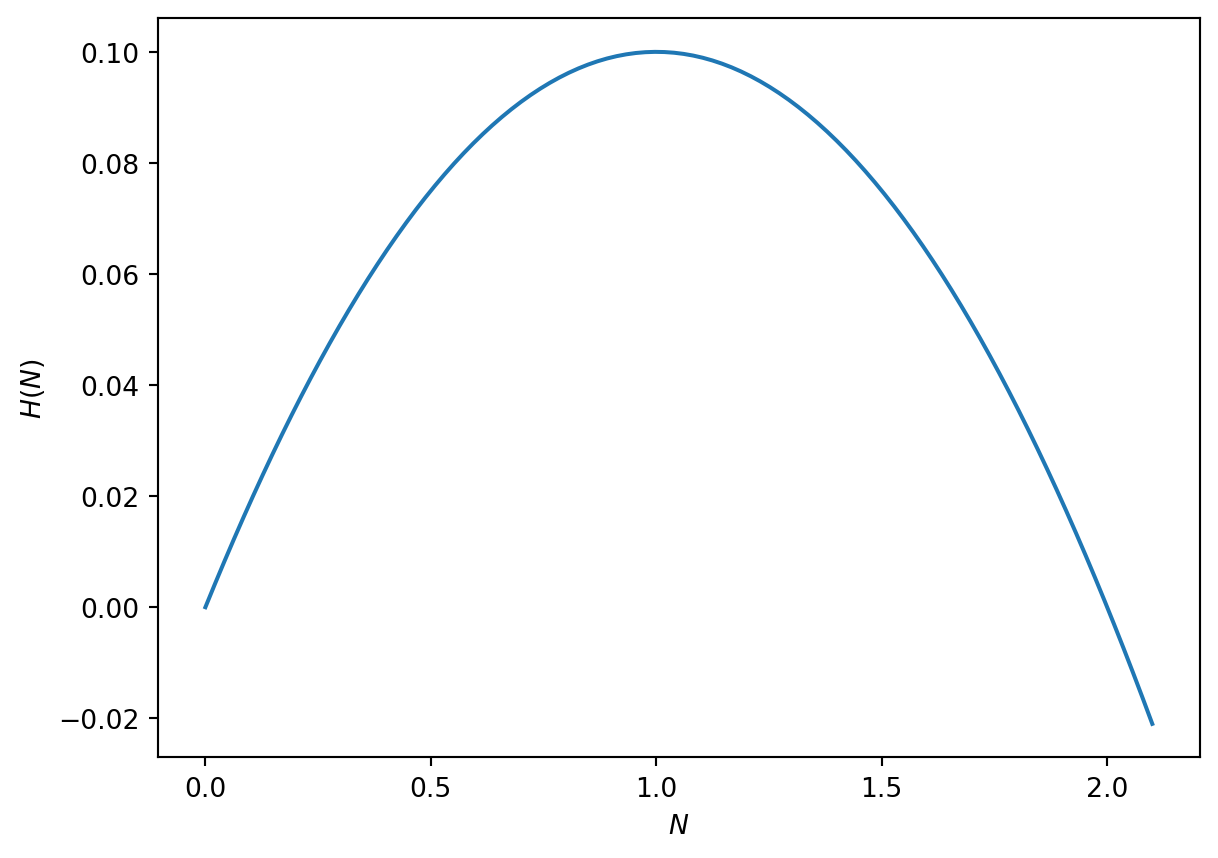
In Figure 4.2 we plot the right-hand side of Equation 4.19. We can qualitatively describe model solutions by considering the arrow along the x axis. Suppose we consider an initial condition with \(0<n_0<1\). Using the graph of \(H(n)\), \(dn/d\tau\) is positive, hence \(n\) increases as a function of time until \(n(\tau)\rightarrow 1\).

import numpy as np
import matplotlib.pyplot as plt
N_max=2.1
K=2
r=0.2
N_vec=np.linspace(0,N_max,100)

rhs=r*N_vec*(1-N_vec/K)
fig, ax = plt.subplots(1)

ax.plot(N_vec, rhs)
plt.xlabel('$N$')
plt.ylabel('$H(N)$')
plt.show()

Figure 4.2: Right-hand side of the logistic ODE

4.3.4 An exact solution

Separation of variables yields \[ \int\frac{ dN}{N(1-\frac{N}{K})}=r\int dt. \tag{4.25}\] Using partial fractions \[ \int\frac{ dN}{N} + \frac{1}{K}\int\frac{ dN}{1-\frac{N}{K}}=r\int dt. \tag{4.26}\] Integration yields, \[ \ln N - \ln\left(1-\frac{N}{K}\right)= \ln \frac{N }{1-\frac{N}{K}} = rt+C. \tag{4.27}\] Hence \[ N=\frac{De^{rt}}{1+\frac{D}{K}e^{rt}} \tag{4.28}\] Given an initial condition \(N(0)=N_0\), we obtain \[ N(t)=\frac{N_0K e^{rt}}{K+N_0(e^{rt}-1)} \tag{4.29}\]

4.3.4.1 Qualitative analysis of the exact solution

As \(t\rightarrow \infty\), \(N\rightarrow K\). At \(t=0\), \(N=N_0\) and that for small \(N_0\ll K\) the initial growth phase is exponential, i.e.  \[ N(t)\sim N_0 e^{rt} \\ \ \ \ \ N_0\ll K, t\ll \frac{1}{r}. \tag{4.30}\]

Note that in almost all the models that we will consider the above method is not an usually an option as the ODE is not explicitly integrable.

4.4 The spruce budworm model

The spruce budworm is a destructive and widely distributed forest defoliator in North America. Massive outbreaks occur periodically and can destroy large quantities of valuable spruce and fir. To understand the outbreak behaviour and develop and management strategies, a series of mathematical models have been developed, beginning with Ludwig et al. (1978). The goal of the models is to explain the qualitative pattern of sudden outbreaks and then a sudden collapse.

4.4.1 Model development

Letting \(N(t)\) represent the population size at time \(t\), it is assumed that budworm exhibits logistic growth and is subject to predation at rate \(p(N)\). A governing ordinary differential equation is given by \[ \frac{dN }{dt}= r_B N\left(1-\frac{N}{K_B}\right)-p(N), \tag{4.31}\] where \[ p(N) =\frac{B N^2}{A^2 +N^2}, \tag{4.32}\] \(r_B\) is the linear growth rate, \(K_B\) is the carrying capacity, \(B\) is the maximum rate of predation and \(A\) is a measure of budworm population where predation switches on (specifically, \(A\) represents the budworm density at which predation is half its maximum value).

It is informative to graph the predation term \[ p(N) =\frac{B N^2}{A^2 +N^2}, \tag{4.33}\] and annotate the parameters \(A\) and \(B\).

There is a root at \(N=0\). In the limit \(N\rightarrow \infty\), \(p \rightarrow B\). Note that for \(N=A\), \(p(A)=B/2\). The derivative is \[ p'(N)=\frac{2BN}{A^2+N^2} - \frac{2BN^3}{(A^2+N^2)^2} = \frac{2BA^2N}{(A^2+N^2)^2} \tag{4.34}\] Thus there is a turning point at \(N=0\) and \(p'>0 \forall N>0\).

4.4.2 Nondimensionalisation

Introducing the (as yet unspecified) dimensional scalings \(\tilde{N}\) and \(\tilde{T}\), the model is nondimensionalised as follows

\[ n=\frac{N}{\tilde{N}} \ \ \ \ \ \ \tau=\frac{t}{\tilde{T}}. \tag{4.35}\]

Changing variables in Equation 4.31 yields

\[ \frac{\tilde{N}}{\tilde{T}}\frac{d n }{d\tau}= r_B \tilde{N}n\left(1-\frac{\tilde{N}n}{K_B}\right)-\frac{B\tilde{N}^2n^2}{A^2+\tilde{N}^2 n^2}. \tag{4.36}\]

After some tidying

\[ \frac{dn }{d\tau}= r_B\tilde{T} n\left(1-\frac{\tilde{N}n}{K_B}\right)-\frac{B\tilde{N} \tilde{T}}{A^2}\frac{n^2}{1+\frac{\tilde{N}^2}{A^2}n^2}. \tag{4.37}\]

A natural scale for cell density in the model is given by the parameter \(A\), as it determines the density of budworm at which predation is half its maximal value. Hence we choose the scaling on the budworm density \[ \tilde{N}=A. \tag{4.38}\] Similarly, a natural time scale for the model is given by
\[ \tilde{T}=A/B. \tag{4.39}\]

Substituting for \(\tilde{N}\) and \(\tilde{T}\) yields \[ \frac{dn }{d\tau}= rn\left(1-\frac{n}{q}\right)-\frac{n^2}{1+n^2} = H(n), \tag{4.40}\] where we define the nondimensional parameters \[ r= \frac{r_B A}{B} \ \ \ \textrm{and} \ \ \ q=\frac{K_B}{A}. \tag{4.41}\]

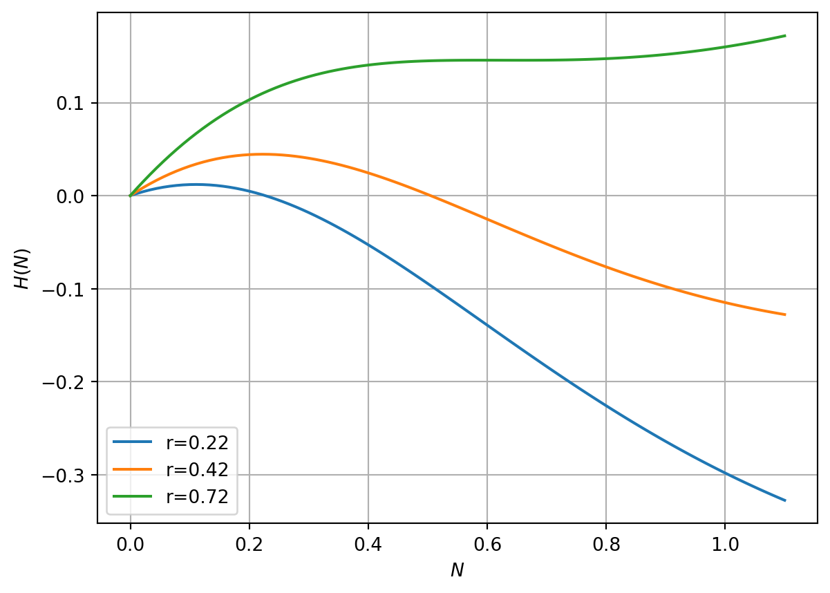
Note that Equation 4.40 has two nondimensional parameters and all variables are dimensionless. See Figure 4.3 for a plot of right-hand side of equation Equation 4.40. What kind of behaviours do you expect to see from the model?

import numpy as np
import matplotlib.pyplot as plt
import scipy
from scipy.integrate import odeint

N_max=1.1
N_0=0.1
q=12
r_1=0.22
r_2=0.42
r_3=0.72

n_vec=np.linspace(0,N_max,100)

def rhssprucebudworm_model(x,t,r,q):

  rhs=r*x*(1-x/q) - x**2/(1+x**2)
  return rhs
def rhssprucebudworm_model_f(x,t,r,q):

  f=r*x*(1-x/q) 
  return f  
def rhssprucebudworm_model_g(x,t,r,q):

  g=x**2/(1+x**2)
  return g  

rhs1=rhssprucebudworm_model(n_vec,0,r_1,q)
rhs2=rhssprucebudworm_model(n_vec,0,r_2,q)
rhs3=rhssprucebudworm_model(n_vec,0,r_3,q)

fig, ax = plt.subplots(1)

ax.plot(n_vec, rhs1,n_vec, rhs2,n_vec, rhs3)
plt.xlabel('$N$')
plt.ylabel('$H(N)$')
plt.legend(['r='+str(r_1),'r='+str(r_2),'r='+str(r_3)])
plt.grid(True)
plt.show()

Figure 4.3: RHS of spr. budworm model

4.4.3 Numerical solutions

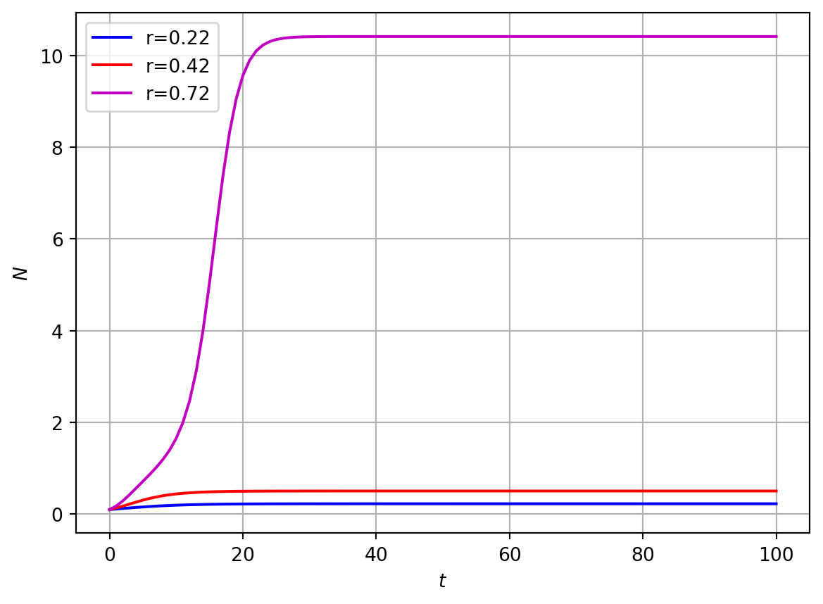
In Figure 4.4 we plot some numerical solutions of Equation 4.40 at different values of the parameter \(r\).

Numerical solutions of Equation 4.40 indicate that there is a single stable steady state when \(r\) is both small and large but for intermediate values of \(r\) there are two stable steady states.

Our goal is to analyse the model and understand why different parameter values yield these strikingly different model behaviours.

# Define time
t = np.linspace(0, 100, 101)

# Numerically solve the ODE for differnet parameter values
sol1 = odeint(rhssprucebudworm_model, N_0, t, args=(r_1, q))
sol2 = odeint(rhssprucebudworm_model, N_0, t, args=(r_2, q))
sol3 = odeint(rhssprucebudworm_model, N_0, t, args=(r_3, q))


# plot results
fig, ax= plt.subplots()
ax.plot(t, sol1, 'b', label='r=' +str(r_1))
ax.plot(t, sol2, 'r', label='r='+str(r_2))
ax.plot(t, sol3, 'm', label='r='+str(r_3))

plt.legend(loc='best')
plt.xlabel('$t$')
plt.ylabel('$N$')

plt.grid()
plt.show()

Figure 4.4: Numerical solution of spr. budworm model

4.4.4 Steady state analysis

Letting \(n^*\) represent steady states of Equation 4.40 yields \[ rn^*(1-\frac{n^*}{q})- \frac{n^*{^2}}{1+n^*{^2}}=0. \tag{4.42}\] Hence either \[ n^*=0, \tag{4.43}\] or \(n^*\) satisfies the cubic equation \[ r\left(1-\frac{n^*}{q}\right)- \frac{n^*}{1+n^*{^2}}=0. \tag{4.44}\] Explicit solutions to such a cubic can be immediately written down but they are cumbersome to work with. We proceed using a graphical/qualitative approach.

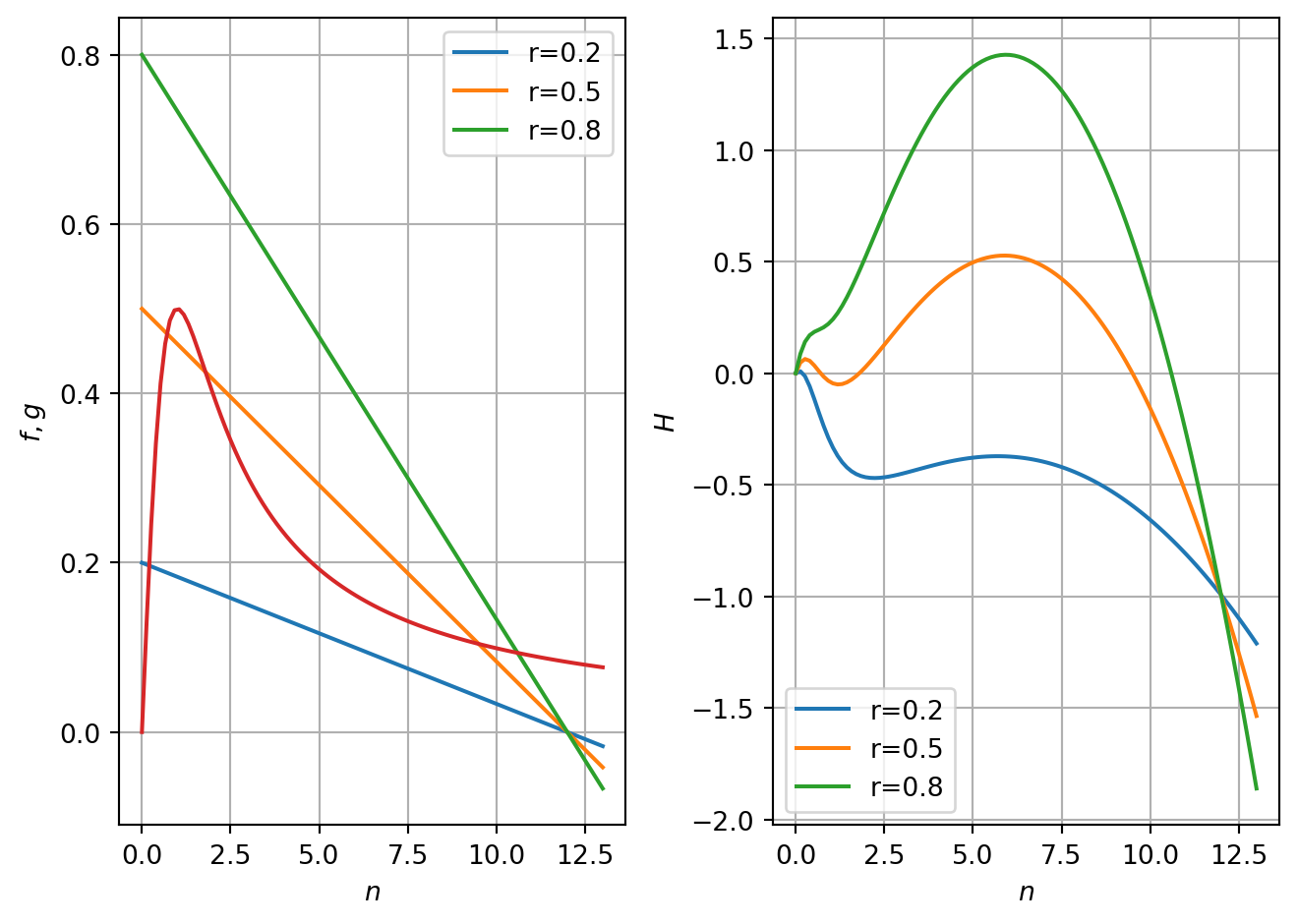
Define \[ f(n^*)=r\left(1-\frac{n^*}{q}\right) \ \ \textrm{and} \ \ g(n^*)=\frac{n^*}{1+n^*{^2}}. \tag{4.45}\] Roots occur for values of \(n^*\) that satisfy \(f=g\).

In Figure 4.5 (a) we fix the parameter \(q=10\) and consider model behaviour as a function of the parameter \(r\). When \(r\gg1\) there is a nonzero steady-state corresponding to \(n^*\gg 1\). When \(r\ll1\) there is a nonzero steady-state corresponding to \(n^*\ll 1\). In the intermediate case there can be three intersection points.

We can use the curve sketching techniques form Tutorial Sheet 1 to sketch \(f\) and \(g\).

\(f\) is linear. There is a root at \(n^*=q\). The derivative is \(-r/q\). \(f(0)\)=r. \(g\) has a unique root at \(n^*=0\). The derivative is \[ g'=\frac{1-n{^*}^2}{(1+n^*)^2}. \tag{4.46}\] There is a turning point at \(n^*=1\). Here \(g=1/2\). As \(n^*\rightarrow \infty\), \(g\rightarrow 0\). \(f'(0)=1\).

4.4.5 Linear stability analysis

The linear stability of the model is determined by the quantity \[ H'(n)=r(1-\frac{2n}{q})-\frac{2{n}}{1+{n}^2} +\frac{2{n}^3}{(1+{n}^2)^2}. \tag{4.47}\]

Hence at the steady state \(n^*=0\) \[ H'(0)=r \tag{4.48}\] and the steady state is linearly unstable.

Given the nonzero steady states have not been calculated explicitly, we proceed using graphical analysis of stability. In Figure 4.5 (b) we plot the right-hand side of Equation 4.40 against \(n\) and examine the cases of large, small and intermediate \(r\) for a given value of \(q\).

When \(r\) is both large and small the nonzero steady state is stable (the derivative at the roots is negative). In the case where three biologically relevant roots exist, the intermediate root is unstable.

import numpy as np
import matplotlib.pyplot as plt
import scipy
from scipy.integrate import odeint




# Define initial condition
N_0=0.1

# Define model parameters
q=12
r_1=0.2
r_2=0.5
r_3=0.8

# Discretise n
N_max=13
n_vec=np.linspace(0,N_max,100)

# Function to compute f and g
def rhssprucebudworm_model_f(x,t,r,q):

  f=r*(1-x/q) 
  return f  
def rhssprucebudworm_model_g(x,t,r,q):

  g=x/(1+x**2)
  return g  

# Compute f for different values of r and g
f_1=rhssprucebudworm_model_f(n_vec,0,r_1,q)
f_2=rhssprucebudworm_model_f(n_vec,0,r_2,q)
f_3=rhssprucebudworm_model_f(n_vec,0,r_3,q)
g=rhssprucebudworm_model_g(n_vec,0,r_1,q)


# Compute H for different values of r
h_1=rhssprucebudworm_model(n_vec,0,r_1,q)
h_2=rhssprucebudworm_model(n_vec,0,r_2,q)
h_3=rhssprucebudworm_model(n_vec,0,r_3,q)


# Plot results
fig, ax = plt.subplots(1,2)

ax[0].plot(n_vec, f_1,n_vec, f_2,n_vec, f_3,n_vec,g)
ax[0].set_xlabel('$n$')
ax[0].set_ylabel('$f,g$')
ax[0].grid(True)
ax[0].legend(['r='+str(r_1),'r='+str(r_2),'r='+str(r_3)])
ax[1].plot(n_vec, h_1,n_vec, h_2,n_vec, h_3)
ax[1].set_xlabel('$n$')
ax[1].set_ylabel('$H$')
ax[1].grid(True)
ax[1].legend(['r='+str(r_1),'r='+str(r_2),'r='+str(r_3)])
plt.tight_layout()
plt.show()

Figure 4.5: RHS of spr. budworm model

4.4.6 Bifurcation analysis

The goal is to identify boundaries of \(rq\) parameter space where the stability changes occur and/or the number of steady states changes.

We can define points in \(rq\) parameter space where bifurcations arise by seeking values of \(n^*\) that satisfy \[ f(n^*)= g(n^*) \ \ \ \ f'(n^*)= g'(n^*). \tag{4.49}\]

The first of these equations yields \[ r(1-\frac{n^*}{q}) = \frac{n^*}{1+n{^*}^{2}}, \tag{4.50}\] and the latter yields \[ -\frac{r}{q}=\frac{1}{1+n{^*}^{2}}-\frac{2n{^*}^{2}}{(1+n{^*})^2} = \frac{1-n{^*}^{2}}{(1+n{^*}^{2})^2}. \tag{4.51}\]

Hence \[ \frac{r}{q}= \frac{n{^*}^{2}-1}{(1+n{^*}^{2})^2}. \tag{4.52}\]

Substituting for \(r/q\) in the first equation yields \[ r-\frac{n{^*}^{2}-1}{(1+n{^*}^{2})^2}n^*=\frac{n^*}{1+n{^*}^{2}}, \tag{4.53}\] which can be written in the form \[ r=\frac{2n{^*}^{3}}{(1+n{^*}^{2})^2}. \tag{4.54}\] Substituting for \(r\) in Equation 4.50 yields \[ \frac{2n{^*}^{3}}{(1+n{^*}^{2})^2}=\frac{2n{^*}^{3}}{(1+n{^*}^{2})^2}\frac{n^*}{q}+\frac{n^*}{1+n{^*}^2} \tag{4.55}\] which, after some algebra, yields \[ q=\frac{2n{^*}^3}{n{^*}^{2}-1}. 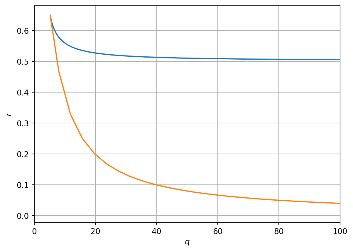\tag{4.56}\] Hence a set of points that define bifurcations where three steady states transform to a single steady state are given in parametric form in \(qr\) parameter space by \[ \left(\frac{2n{^*}^3}{n{^*}^{2}-1},\frac{2n{^*}^{3}}{(1+n{^*}^{2})^2}\right) \ \ \ \ \ \ \ n^*>1. \tag{4.57}\]

# Function to compute bifurcation values of r and q as a function of n_star
def Computerq(x):
  q_n_star=2*x**3/(x**2-1)
  r_n_star=2*x**3/(1+x**2)**2
  return  r_n_star,q_n_star

# Define different domains of n
n_s_1=np.linspace(1,np.sqrt(3),100)
n_s_2=np.linspace(np.sqrt(3),200,100)

# Compute r and q
r_1,q_1=Computerq(n_s_1)
r_2,q_2=Computerq(n_s_2)

# Plot results
fig, ax = plt.subplots(1)

ax.plot(q_1, r_1,q_2, r_2)
plt.xlabel('$q$')
plt.ylabel('$r$')
ax.set_xlim([0, 100])
plt.grid(True)

plt.show()

Figure 4.6: Bifurcations in the rq plane

By varying values of \(n^*\) in Figure 4.6 we plot a region of instability. Note for example that \(q\rightarrow \infty\) as \(n^*\rightarrow 1\) and as \(n^*\rightarrow \infty\). Note also that in these limits \(r\) must take the value 1/2 and 0, respectively.

We can show that the cusp in Figure 4.6 is given by \[ \left(q,r\right)=\left(3^{\frac{3}{2}},\left(\frac{\sqrt{3}}{2}\right)^3\right). \tag{4.58}\]

Note that \(r\) is a decreasing function of \(q\) for \(1<n^*<\sqrt{3}\) but that \(r\) is an increasing function of \(n^*\) for \(\sqrt{3}<n^*<\infty\). This can be shown by finding the turning points of \(r\) w.r.t \(n^*\), i.e. Given that \[ r=\frac{2n{^*}^{3}}{(1+n{^*}^{2})^2}, \tag{4.59}\] differentiation with respect to \(n^*\) yields \[ \frac{dr}{dn^*}=\frac{6{n^*}^2}{(1+n^*)^2} - \frac{8n{^*}^4}{(1+n^*)^3}. \tag{4.60}\] The turning point satisfies \[ \frac{6{n^*}^2}{(1+n^*)^2} - \frac{8n{^*}^4}{(1+n^*)^3}=0 \tag{4.61}\] Solving for \(n^*\) yields \[ 6(1+{n^*}^2) - 8n{^*}^2=0 \tag{4.62}\] Hence \[ n^*=\sqrt{3}. \tag{4.63}\] Thus there is a turning point that minimises \(r\) at \(n^*=\sqrt{3}\).

Substitution for this value of \(n^*\) yields \[ \left(q,r\right)=\left(3^{\frac{3}{2}},\left(\frac{\sqrt{3}}{2}\right)^3\right). \tag{4.64}\] See Figure 4.6.

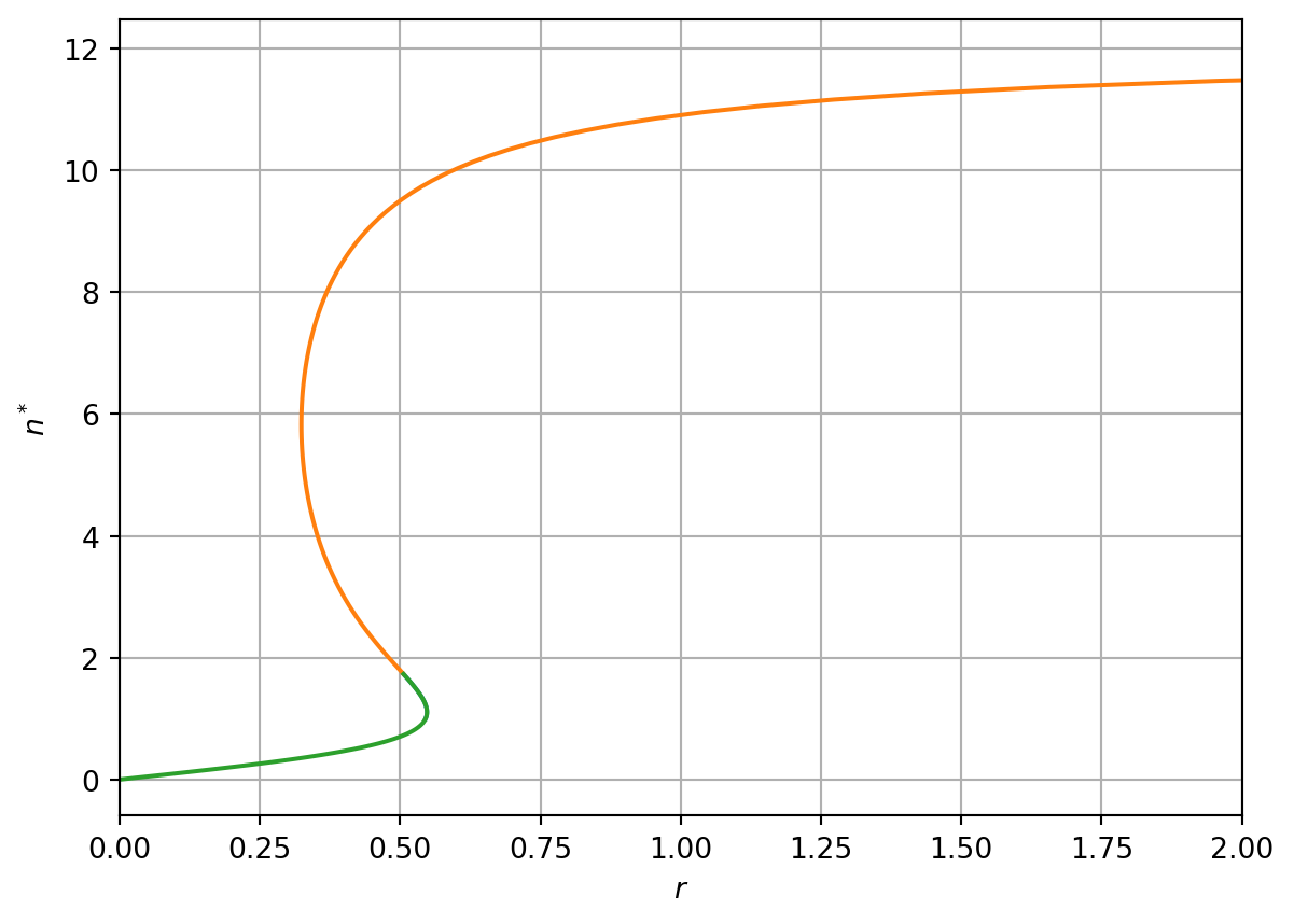
4.4.7 Hysteresis

Finally, rearranging the steady-state equation \[ r(1-\frac{n^*}{q}) = \frac{n^*}{1+n{^*}^{2}}, \] we obtain \[ r = \frac{n^*}{(1+n{^*}^{2})(1-\frac{n^*}{q})}. \tag{4.65}\]

Considering \(n^*<q\) we compute \(r\); plotting \(n^*\) against \(r\) yields the bifurcation curve presented in Figure 4.7.

# Compute r as a function of n
def Computern(x,q):
  r=x/((1+x**2)*(1-x/q))
  return  r

# Define different domains of n for plotting 
q=12
n_s_1=np.linspace(1,np.sqrt(3),100)
n_s_2=np.linspace(np.sqrt(3),0.99*q,100)
n_s_3=np.linspace(0,np.sqrt(3),100)


# Evaluate r
r_1=Computern(n_s_1,q)
r_2=Computern(n_s_2,q)
r_3=Computern(n_s_3,q)


# Plote results
fig, ax = plt.subplots(1)

ax.plot(r_1, n_s_1,r_2, n_s_2,r_3,n_s_3)
plt.xlabel('$r$')
plt.ylabel('$n^*$')
ax.set_xlim([0, 2])
plt.grid(True)

plt.show()

Figure 4.7: Bifurcations in the rq plane

A system exhibiting hysteresis shows a response to an increases in a control parameter that is not exactly reversed when the parameter is decreased. We can show that the spruce budworm model exhibits hysteresis by considering the argument below.

import numpy as np
import math
import matplotlib.pyplot as plt
from matplotlib import animation
from IPython.display import HTML, display
import os

fmt = os.getenv("QUARTO_FORMAT")

plt.rcParams.update({
    "text.usetex": True,
    "text.latex.preamble": r"\usepackage{amsmath}\usepackage{xcolor}"
})

# -----------------------
# Parameters
# -----------------------
q = 12
n_vec = np.linspace(0, 13, 200)
rmax = 0.8
rmin = 0.05

# -----------------------
# Functions
# -----------------------
def f_func(x, r):
    return r * (1 - x / q)

def g_func(x):
    return x / (1 + x**2)

g = g_func(n_vec)

# -----------------------
# Figure set up
# -----------------------
fig, ax = plt.subplots(2, 1, figsize=(6, 9))

fig.suptitle("Hysteresis of spruce budworm model")

line_f, = ax[0].plot(n_vec, f_func(n_vec, 0.1), label="f")
line_g, = ax[0].plot(n_vec, g, label="g")
pts, = ax[0].plot([], [], "ro")

line_up, = ax[1].plot([], [], 'b-', label="r increasing")
line_down, = ax[1].plot([], [], 'r-', label="r decreasing")

ax[0].set_xlabel("n")
ax[0].set_ylabel("f, g")
ax[0].legend()

ax[1].set_xlabel("r")
ax[1].set_ylabel("n*")
ax[1].set_xlim(rmin, rmax)
ax[1].set_ylim(0, 11)
ax[1].legend(loc="upper left", frameon=True)

# -----------------------
# Storage
# -----------------------
r_up_hist = []
n_up_hist = []

r_down_hist = []
n_down_hist = []

# -----------------------
# Root finding
# -----------------------
def find_roots(r):
    y = f_func(n_vec, r) - g_func(n_vec)

    roots = []
    for i in range(len(n_vec) - 1):
        if y[i] * y[i + 1] < 0:
            n1, n2 = n_vec[i], n_vec[i + 1]
            y1, y2 = y[i], y[i + 1]
            root = n1 - y1 * (n2 - n1) / (y2 - y1)
            roots.append(root)

    return roots

# -----------------------
# Hysteresis sweep
# -----------------------
r_up = np.linspace(rmin, rmax, 120)
r_down = np.linspace(rmax, rmin, 120)
r_vals = np.concatenate([r_up, r_down])

# -----------------------
# Clear bottom plot
# -----------------------
def clear_bottom():
    r_up_hist.clear()
    n_up_hist.clear()
    r_down_hist.clear()
    n_down_hist.clear()

    line_up.set_data([], [])
    line_down.set_data([], [])

    fig.canvas.draw_idle()

# -----------------------
# Update function
# -----------------------
prev_r = None
def update(r):

    global prev_r

    # direction detection
    if prev_r is None:
        direction = 1
    else:
        direction = 1 if r >= prev_r else -1

    prev_r = r

    # update f curve
    line_f.set_ydata(f_func(n_vec, r))

    roots = find_roots(r)

    if roots:
        if direction == 1:
            chosen = min(roots)
            r_up_hist.append(r)
            n_up_hist.append(chosen)
        else:
            chosen = max(roots)
            r_down_hist.append(r)
            n_down_hist.append(chosen)

        pts.set_data([chosen], [f_func(chosen, r)])
    else:
        pts.set_data([], [])

    # update hysteresis curves
    line_up.set_data(r_up_hist, n_up_hist)
    line_down.set_data(r_down_hist, n_down_hist)

    ax[0].set_title(f"r = {r:.2f}")

    fig.canvas.draw()
    fig.canvas.flush_events()

    # Clear bottom plot after loop
    if np.isclose(r, r_vals[-1]):
        clear_bottom()

    return line_f, pts, line_up, line_down

# -----------------------
# Animation
# -----------------------
ani = animation.FuncAnimation(fig, update, frames=r_vals, interval=50, blit=True)

if fmt == "html" or fmt is None:
  display(HTML(ani.to_html5_video()))
  plt.close(fig)
else:
  # ---- Render final frame for PDF ----
  update(total_frames + final_wait - 1)
  plt.show()

Figure 4.8: Animation demonstrating hysteresis as \(r\) increases (picks left stable critical point) and decreases (picks right stable critical point).

Suppose \(r\) is initially small (\(r<r_1\)). There is only one steady-state and any initial condition will converge towards it.

Suppose we increase the value of the parameter \(r\). There will be a critical value of \(r\) (\(r=r_1\))where a second stable steady-state arises and the model enters the bistable regime, where there are two possible stable steady-states. Given the system was originally in the first stable steady state, it will remain there.

Suppose we continue to increase \(r\). Eventually we reach critical value of \(r\) (\(r=r_2\)) where the first stable steady state is lost and there is again only one stable steady-state.

Suppose we now decrease the parameter \(r\) below the threshold \(r=r_2\). The system again enters the bistable regime but as the second solution is stable, it remains the solution.

Suppose we continue to decrease \(r\) until eventually \(r<r_1\). We return to the case where the system has only a single stable steady state.

4.5 Harvesting

By introducing terms that represent harvesting, population models can be used to investigate management strategies for resource management. The modelling problem is to maximise the sustained yield.

Consider a model for logistic growth supplemented with a harvesting term \[ \frac{dN}{dt}=rN\left(1-\frac{N}{K}\right) - EN. \tag{4.66}\] The term \(EN\) is the harvesting yield per unit time and the constant \(E\) represents the harvesting effort.

Steady states satisfy \[ rN^*\left(1-\frac{N^*}{K}\right) - EN^*=0 \tag{4.67}\] Thus either \(N^*=0\) or \[ \left(1-\frac{N^*}{K}\right) -E=0 \tag{4.68}\] Hence \[ N^*=K(1-\frac{E}{r}). \tag{4.69}\] Note that this is positive only if \[ E<r. \tag{4.70}\] Thus if the harvesting rate exceeds the linear growth rate the only steady state corresponds to extinction.

The yield is, \[ Y(E)=EN^*=EK(1-\frac{E}{r}) \tag{4.71}\]

To maximise the yields we differentiate with respect to \(E\). \[ \frac{dY}{dE} = K - 2\frac{EK}{r}. \tag{4.72}\] Thus the maximum yield is identified by setting \[ \frac{dY}{dE} = K - 2\frac{EK}{r}=0. \tag{4.73}\] THe maximum occurs at harvesting rate \[ E_c=\frac{r}{2}. \tag{4.74}\] The maximum yield is \[ E^*=\frac{rK}{4}. \tag{4.75}\]

We identify the time scale over which stocks return to steady state by linearising about the steady state \(N^*=K(1-E/r)\), hence \[ \frac{d \hat{N}}{dt} = (E-r)\hat{N}. \tag{4.76}\] Hence the recovery time scale is \[ T_R(E)=O(\frac{1}{r-E}). \tag{4.77}\] As the harvesting rate approaches the linear growth rate \(r\), not only does the steady state population tend to zero but the timescale for stocks to recover tends to infinity.

4.6 Delay differential equation models

Consider a model of the form \[ \frac{dN}{dt}=H(N(t),N(t-T)), \tag{4.78}\] such that the right-hand side now depends on the value \(N\) not just at time \(t\) but also at some delay time \(t-T\). We now need to prescribe initial conditions of the form \[ N(t)=f(t), \quad -T<t\leq0. \tag{4.79}\]

Consider a simple case of a linear model \[ \frac{dN}{dt}=-N(t-T). \tag{4.80}\] A steady state, \(N^*\), is defined such that \(N(t)=N(t-T)=N^*\). Hence \[ 0=-kN^*. \tag{4.81}\] The only steady state is \(N^*=0\).

To compute the linear stability we consider solution of the linearised equation of the form \[ N(t)=e^{\lambda t}. \tag{4.82}\] Hence \[ N(t-T)=e^{\lambda (t-T)}. \tag{4.83}\]

Substitution yields \[ \lambda e^{\lambda t} = - e^{\lambda (t-T)}. \tag{4.84}\] Hence the eigenvalue, \(\lambda\), satisfies a transcendental equation \[ \lambda=-e^{-\lambda T}. \tag{4.85}\] This equation has no solutions for \(\lambda \in \Re^+\). Hence any steady-states with real eigenvalues are linearly stable.

Now consider solutions \(\lambda \in \mathbb{C}\). Let \(\lambda=\mu+i\omega\). Substitution yields \[ \mu+i\omega = -e^{-\mu T}(\cos(\omega T)-i \sin(\omega T)). \tag{4.86}\] Hence \[ \mu=-\cos(\omega T)e^{-\mu T} \tag{4.87}\] and \[ \omega = \sin(\omega T)e^{-\mu T}. \tag{4.88}\]

For linear stability of the steady state it is required that \(\mu <0\).

If \(\omega\) is a solution of Equation 4.87 and Equation 4.88 then so is \(-\omega\). Hence w.l.o.g we consider the case \(\omega>0\).

Consider \(\mu=0\) in Equation 4.87. This implies \[ \omega T=\frac{\pi}{2} + 2n\pi, \quad n \in Z. \tag{4.89}\] We consider the smallest positive root, i.e. \(n=0\), as we want to consider the smallest value of delay time, \(T\), at which instability arises.

Note \(\mu<0\) for \[ \omega T< \frac{\pi}{2}. \tag{4.90}\]

On the stablity boundary, \(\mu=0\). Upon substitution in Equation 4.88 \[ \omega = \sin(\frac{\pi}{2})=1. \tag{4.91}\]

Hence the steady state is linearly stable for \[ T< \frac{\pi}{2}. \tag{4.92}\]

4.7 References

Ludwig, Donald, Dixon D Jones, Crawford S Holling, et al. 1978. “Qualitative Analysis of Insect Outbreak Systems: The Spruce Budworm and Forest.” Journal of Animal Ecology 47 (1): 315–32.